Ranking and flow#
This is the first type of analysis we’ll talk about that really only makes sense for directed networks. There are a few ways to motivate a similar kind of analysis, which I’ll put under the umbrella of “ranking” or “flow” through a directed network.
Let’s say we have a network, where directed edges represent some kind of “dominance” relationship. An example could be a network of teams, where edges represent a victory by team \(i\) over team \(j\). Or, it could be a network of individual animals, and edges represent an interaction where an ecologist watched one animal somehow dominate another. Or, it could be a food web, where an edge represents that organism \(i\) consumes organism \(j\).
Another perspective is that we just have a directed network, and we want to understand how information/signal/etc flows through it. An example would be a network of neurons (connectome), and we might want to understand which neurons are closer to sensory input and which neurons are closer to motor output.
NCAA Football network#
Let’s start by considering the ranking problem, where an edge from \(i\) to \(j\) represents a victory of team \(i\) over team \(j\). We could use weights if we want (for something like a score differential, say). I’ll stick with this nomenclature for this discussion, but note that it could apply to something other than teams and games.
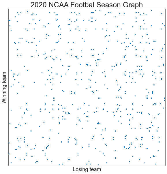
Below, I’ll create a network from the 2020 NCAA Football season.
import pandas as pd
import numpy as np
import re
import matplotlib.pyplot as plt
from graspologic.plot import adjplot
import seaborn as sns

# REF: https://www.sports-reference.com/cfb/years/2020.html
schedule = pd.read_csv("networks-course/data/sports/ncaa_football_2020.csv")


def filt(string):
    return re.sub(r"\([0123456789]*\) ", "", string)


vec_filt = np.vectorize(filt)

schedule["Winner"] = vec_filt(schedule["Winner"])
schedule["Loser"] = vec_filt(schedule["Loser"])


unique_winners = np.unique(schedule["Winner"])
unique_losers = np.unique(schedule["Loser"])
teams = np.union1d(unique_winners, unique_losers)
n_teams = len(teams)

adjacency_df = pd.DataFrame(
    index=teams, columns=teams, data=np.zeros((n_teams, n_teams))
)

for idx, row in schedule.iterrows():
    winner = row["Winner"]
    loser = row["Loser"]
    adjacency_df.loc[winner, loser] += 1

remove_winless = False
n_wins = adjacency_df.sum(axis=1)
if remove_winless:
    teams = teams[n_wins > 0]
    n_wins = adjacency_df.sum(axis=1)
adjacency_df = adjacency_df.reindex(index=teams, columns=teams)

n_teams = len(teams)

sns.set_context("talk")

ax, _ = adjplot(adjacency_df.values, plot_type="scattermap", sizes=(10, 10), marker="s")
ax.set_title("2020 NCAA Footbal Season Graph", fontsize=25)
ax.set(ylabel="Winning team")
ax.set(xlabel="Losing team")

print(f"Number of teams {n_teams}")
Number of teams 143
import networkx as nx
from graspologic.plot import networkplot
from graspologic.partition import leiden

g = nx.from_pandas_adjacency(adjacency_df, create_using=nx.DiGraph)
g_sym = nx.from_pandas_adjacency(adjacency_df + adjacency_df.T, create_using=nx.Graph)
pos = nx.kamada_kawai_layout(g)

nodelist = adjacency_df.index
node_data = pd.DataFrame(index=nodelist)

xs = []
ys = []
for node in adjacency_df:
    xs.append(pos[node][0])
    ys.append(pos[node][1])
xs = np.array(xs)
ys = np.array(ys)

node_data["x"] = xs
node_data["y"] = ys

partition_map = leiden(g_sym, trials=100, random_seed=8888)
labels = np.vectorize(partition_map.get)(nodelist)

node_data["leiden_labels"] = labels

palette = dict(zip(np.unique(labels), sns.color_palette("tab10")))

ax = networkplot(
    adjacency_df.values,
    node_data=node_data.reset_index(),  # bug in this function requires the .reset_index
    x="x",
    y="y",
    node_alpha=1.0,
    edge_alpha=1.0,
    edge_linewidth=0.6,
    node_hue="leiden_labels",
    node_kws=dict(s=100, linewidth=2, edgecolor="black"),
    palette=palette,
)
_ = ax.axis("off")
fig = ax.get_figure()
_ = fig.set_facecolor("white")

from scipy.interpolate import splprep, splev
from scipy.spatial import ConvexHull


def fit_bounding_contour(points, s=0, per=1):
    hull = ConvexHull(points)
    boundary_indices = list(hull.vertices)
    boundary_indices.append(boundary_indices[0])
    boundary_points = points[boundary_indices].copy()

    tck, u = splprep(boundary_points.T, u=None, s=s, per=per)
    u_new = np.linspace(u.min(), u.max(), 1000)
    x_new, y_new = splev(u_new, tck, der=0)
    return x_new, y_new


def draw_bounding_contour(points, color=None, linewidth=2):
    x_new, y_new = fit_bounding_contour(points)
    ax.plot(x_new, y_new, color=color, zorder=-1, linewidth=linewidth, alpha=0.5)
    ax.fill(x_new, y_new, color=color, zorder=-2, alpha=0.1)


for group_name, group_data in node_data.groupby("leiden_labels"):
    points = group_data[["x", "y"]].values
    if len(points) > 2:
        draw_bounding_contour(points, color=palette[group_name])
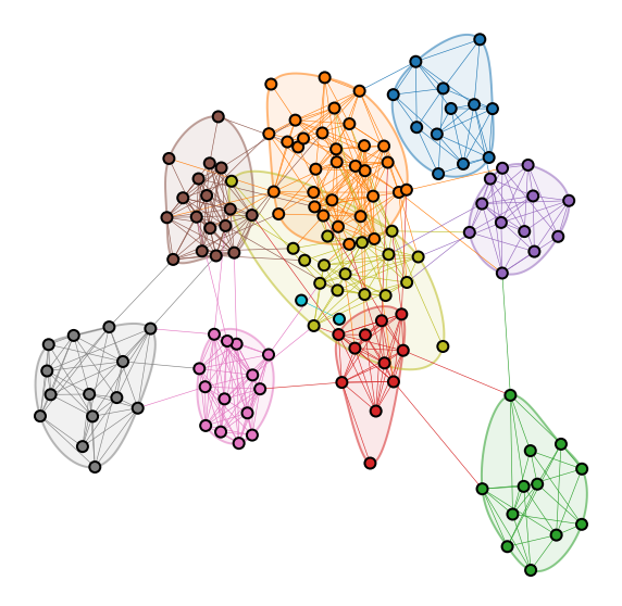
Question
What do you think the communities I plot above correspond to?
adjacency_df.index[labels == 2].values
array(['Arizona', 'Arizona State', 'California', 'Colorado', 'Oregon',
       'Oregon State', 'Southern California', 'Stanford', 'UCLA', 'Utah',
       'Washington', 'Washington State'], dtype=object)
Simple and eigenvector rankings#
Question
What is perhaps the simplest way to say which teams are doing well in a given year, say just given the outcome of each game in a season?
For the metric you just described, how can we compute it using the adjacency matrix?
Let \(r_0\) be the vector of all ones. Note now that
is calculating the number of wins for each team if the adjacency matrix just has counts of wins in its elements.
n_wins = np.sum(adjacency_df, axis=1)
node_data["n_wins"] = n_wins
n_wins.sort_values(ascending=False)
Alabama              13.0
Brigham Young        11.0
Coastal Carolina     11.0
Notre Dame           10.0
Clemson              10.0
                     ...
Nevada-Las Vegas      0.0
New Mexico State      0.0
North Alabama         0.0
Northern Illinois     0.0
Abilene Christian     0.0
Length: 143, dtype: float64
Note that it is easy to have ties in this ranking. Also, teams could play different numbers of games in some leagues/situations, which we might want to account for. With \(d_i\) being the total degree of node \(i\) (numbers of wins AND losses), and \(D\) being a matrix with these degrees on the diagonal we could make an adjustment like
Question
How can we interpret this new ranking scheme in terms of wins/losses for a given team?
n_games = np.sum(adjacency_df, axis=0) + np.sum(adjacency_df, axis=1)
win_rates = n_wins / n_games
node_data["win_rate"] = win_rates
win_rates.sort_values(ascending=False)
Alabama              1.000000
Tarleton State       1.000000
Brigham Young        0.916667
Coastal Carolina     0.916667
Louisiana            0.909091
                       ...
Mercer               0.000000
Missouri State       0.000000
Nevada-Las Vegas     0.000000
New Mexico State     0.000000
Abilene Christian    0.000000
Length: 143, dtype: float64
from scipy.stats import rankdata


def rank_to_order(key):
    node_data[f"{key}_order"] = rankdata(node_data[key])


rank_to_order("win_rate")
In a league like NCAA where not all teams play each other, this ranking does not account for strength of schedule. Perhaps our ranking scheme should account not just for the number or proportion of wins, but also the quality of the teams that we beat. We can account for this by instead, say, calculating the sum of the number of wins of the teams that team \(i\) beat:
I love this quote from Keener [1] (I have changed the mathematical notation only to match ours):
“I have heard it suggested by a nationally prominent football coach that \(A^2 r_0\) should be used to determine a national champion… Of course, he did not express his scheme in mathematical notation, and, therefore, did not see the obvious generalization of using \(A^s r_0\) with large \(s\).”
Earlier in the course, we talked about power iteration. This is a method for calculating the principal eigenvector/eigenvalue of a matrix. It is based on the idea that, as \(s\) goes to infinity,
where here \(r\) is now the principal eigenvector of \(A\).
Note
Fun fact: this positive principal eigenvector is only guaranteed to exist when the network is fully (weakly) connected (see the Perron-Frobenius theorem or Keener [1]). But this is kind of cool - if the network weren’t fully connected, it would mean that we can divide the set of teams into groups that never play each other - in other words, they are different leagues! So this breaks down exactly when we’d expect it to.
A = adjacency_df.values


def eig(A):
    evals, evecs = np.linalg.eig(A)
    sort_inds = np.argsort(-evals)
    evals = evals[sort_inds]
    evecs = evecs[:, sort_inds]
    return evals, evecs


evals, evecs = eig(A)
principal_evec = np.abs(evecs[:, 0])
eigvec_ranking = pd.Series(index=adjacency_df.index, data=principal_evec)
node_data["evec_rank"] = eigvec_ranking
rank_to_order("evec_rank")
eigvec_ranking.sort_values(ascending=False)
Oklahoma                 0.446343
Iowa State               0.439824
Oklahoma State           0.328123
Texas                    0.258606
Alabama                  0.239614
                           ...
Florida International    0.000000
Tarleton State           0.000000
Temple                   0.000000
Ohio                     0.000000
Abilene Christian        0.000000
Length: 143, dtype: float64
from matplotlib import colors


def plot_network_color_scaled(key):
    levels = list(np.sort(node_data[key].unique()))
    cmap = sns.color_palette("Blues", as_cmap=True)
    vmin = np.min(levels)
    norm = colors.Normalize(vmin=0.3 * vmin)
    palette = dict(zip(levels, cmap(norm(levels))))

    ax = networkplot(
        adjacency_df.values,
        node_data=node_data.reset_index(),  # bug in this function requires the .reset_index
        x="x",
        y="y",
        node_alpha=1.0,
        edge_alpha=1.0,
        edge_linewidth=0.6,
        node_hue=key,
        node_size=key,
        node_sizes=(30, 300),
        node_kws=dict(linewidth=1.5, edgecolor="black"),
        palette=palette,
        edge_kws=dict(color=sns.color_palette()[0]),
    )
    ax.axis("off")
    return ax
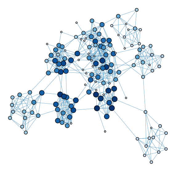
plot_network_color_scaled("evec_rank_order")
<AxesSubplot:xlabel='x', ylabel='y'>
Brief aside#
Watch what happens if you use the normalized adjacency / Laplacian here instead.
k = np.sum(A, axis=0) + np.sum(A, axis=1)
D_inv = np.diag(1 / k)
P = D_inv @ A

evals, evecs = eig(P)
principal_evec_lap = np.abs(evecs[:, 0])
eigvec_ranking_lap = pd.Series(index=adjacency_df.index, data=principal_evec_lap)
node_data["evec_rank_lap"] = eigvec_ranking_lap
rank_to_order("evec_rank_lap")
eigvec_ranking_lap.sort_values(ascending=False)[:10]
Stanford               0.432102
Oregon                 0.394296
Washington             0.365687
Southern California    0.337310
Utah                   0.330062
California             0.253709
Colorado               0.249628
Oregon State           0.238261
Washington State       0.153309
Arizona State          0.153309
dtype: float64
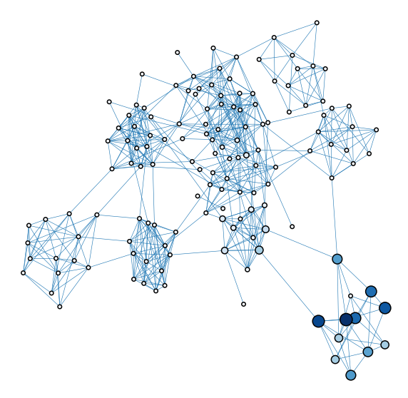
plot_network_color_scaled(key="evec_rank_lap")
<AxesSubplot:xlabel='x', ylabel='y'>
Signal flow / laplacian ranking#
There is another, similar but distinct notion of ranking which is related to the network Laplacian. Let’s write down a couple of definitions:
\(W \in \mathbb{R}^{n \times n}\): \(\frac{A + A^T}{2}\), the symmetrized adjacency matrix
\(\Delta \in \mathbb{R}^{n \times n}\): an antisymmetric matrix, which we will specify later
\(z \in \mathbb{R}^{n}\): the vector of signal flows for each node \(\{1, 2, ... ,n\}\)
Defining an energy (objective) function#
We start by defining an energy function:
Let \(E_0 = \frac{1}{2} \sum_{i, j = 1}^n w_{ij} x_{ij}^2\)
Note that \(\frac{1}{2} \sum_{i, j = 1}^n w_{ij} (z_i - z_j)^2\) is related to the unnormalized graph laplacian: \(L = D - W\)
Let \(d_i = \sum_{j = 1}^n w_{ij}\), the degree of node \(i\). Since \(W\) is symmetric
Now, consider the term
define \(b_i = \sum_{j=1}^n w_{ij}x_{ij}\). Now the above reduces to
where \(E_0\) is the remaining constant (which does not depend on \(z\)).
Solving for \(z\)#
Taking the derivative of \(E(z)\),
Setting equal to 0,
\(L\) is singular. To see this, recall that
Let \(x\) be the vector of all ones, then
Thus, \(Lx = 0 = 0x\) so the vector of all ones is an eigenvector of \(L\) with eigenvalue \(0\), so \(L\) is not invertible.
However, we can solve
via the Moore-Penrose inverse of \(L\), \(L^\dagger\).
The Moore-Penrose inverse yields the unique solution to \(\min_z \| Lz - b \|_2\) with minimum 2-norm. However, there are many solutions, all of the form
where \(y \in Null(L)\). What is in \(Null(L)\)? Any vector spanned by the vector of all ones, as shown above! This means that all of the values of the signal flow vector \(z\) could be shifted by a constant and the value of the objective function \(E(z)\) would remain the same. Signal flow is not an absolute measure, but rather, a measure of where a node lives in the graph relative to its peers.
Defining \(\Delta\)#
What we have seen is that
is minimized by \(z = L^\dagger b\), where \(b\) is a vector such that \(b_i = \sum_{j=1}w_{ij}\delta_{ij}\)
\(\Delta\) can be whatever we choose, as long as it is antisymmetric. One choice used in Varshney et al. 2011 is \(\delta_{ij} = sgn(A_{ij} - A_{ji})\) This choice makes some intuitive sense.
Some intuition#
Considering a single pair of nodes, \(i, j\), the energy function looks like
If \(A_{ij} > A_{ji}\), then node \(i\) projects more strongly to \(j\) than \(j\) does to it. \(sgn(A_{ij} - A_{ji})\) returns 1, and so the optinal configuration of \(z_i\) and \(z_j\) is to have \(z_i = z_j + 1\).
\(z\) is chosen by weighting each of these terms by the average projection weight \(w_{ij}\), and finding the solution \(z\) which minimizes these terms over all \(i, j\) pairs.
W = (A + A.T) / 2

D = np.diag(np.sum(W, axis=1))

L = D - W

b = np.sum(W * np.sign(A - A.T), axis=1)
L_dagger = np.linalg.pinv(L)  # this is the Moore-Penrose inverse
z = L_dagger @ b

signal_flow_rank = pd.Series(data=z, index=adjacency_df.index)
node_data["sf_rank"] = signal_flow_rank - signal_flow_rank.min()
rank_to_order("sf_rank")
signal_flow_rank.sort_values(ascending=False)
Alabama                  2.072149
Texas A&M                1.655812
Georgia                  1.578020
Ohio State               1.527953
Ball State               1.502823
                           ...
Stephen F. Austin       -1.256503
Abilene Christian       -1.290551
Houston Baptist         -1.335099
Florida International   -1.531728
Chattanooga             -1.636243
Length: 143, dtype: float64
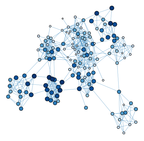
plot_network_color_scaled("sf_rank_order")
<AxesSubplot:xlabel='x', ylabel='y'>
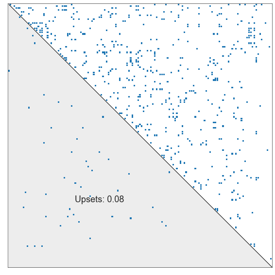
Upset minimization or minimum violations ranking#
Now, let’s switch gears entirely, and talk about a completely different perspective on the ranking problem. I’ll start by making a very simple claim: a good ranking of my teams is one in which, as often as is possible, the higher ranked team beat the lower ranked one.
How can we write what we are after mathematically? If \(P\) is a permutation matrix, then we can write:
In other words, this is the sum of the upper triangular elements of some permuted version of the adjacency matrix.
Question
Let’s say we trust this ordering of the teams under some \(P\). What does the sum of the upper triangle represent? The sum of the lower triangle?
Question
Can you think of a way to formulate the optimization problem above, using the tools that we talked about in this course?
from graspologic.match import GraphMatch

adj = adjacency_df.values

# constructing the match matrix
match_mat = np.zeros_like(adj)
triu_inds = np.triu_indices(len(match_mat), k=1)
match_mat[triu_inds] = 1

# running graph matching
np.random.seed(8888)
gm = GraphMatch(n_init=200, max_iter=150, eps=1e-6, n_jobs=-2)
gm.fit(match_mat, adj)
gm_perm_inds = gm.perm_inds_
adj_matched = adj[gm_perm_inds][:, gm_perm_inds]
upsets = adj_matched[triu_inds[::-1]].sum()
n_games = adj_matched.sum()

gm_ranking_teams = teams[gm_perm_inds]

gm_rank_order = pd.Series(
    index=gm_ranking_teams,
    data=len(teams) + 1 - np.arange(1, len(teams) + 1, dtype=int),
)
node_data["gm_rank_order"] = gm_rank_order

print(f"Number of games: {n_games}")
print(f"Number of non-upsets (graph matching score): {gm.score_}")
print(f"Number of upsets: {upsets}")
print(f"Upset ratio: {upsets/n_games}")

gm_rank_order.sort_values(ascending=False)
Number of games: 569.0
Number of non-upsets (graph matching score): 524.0
Number of upsets: 45.0
Upset ratio: 0.07908611599297012
Liberty             143
Coastal Carolina    142
Alabama             141
Louisiana           140
Ohio State          139
                   ...
Tarleton State        5
Missouri State        4
Chattanooga           3
Mercer                2
New Mexico State      1
Length: 143, dtype: int64
def plot_sorted_adjacency(
    adj,
    shade_upsets=True,
    ax=None,
    perm_inds=None,
    label=False,
    plot_type="scattermap",
    title="",
):
    if perm_inds is not None:
        adj = adj[perm_inds][:, perm_inds]
    if plot_type == "scattermap":
        ax, _ = adjplot(adj, plot_type="scattermap", sizes=(10, 10), marker="s", ax=ax)
    else:
        ax, _ = adjplot(adj, plot_type="heatmap", ax=ax)

    triu_inds = np.triu_indices(len(match_mat), k=1)
    n_upsets = adj[triu_inds[::-1]].sum()
    n_games = adj.sum()
    p_upset = n_upsets / n_games

    ax.set_title(title)

    ax.plot([0, n_teams], [0, n_teams], linewidth=1, color="black", linestyle="-")
    if label:
        ylabel = r"$\leftarrow$ Ranked low         "
        ylabel += "Winning team           "
        ylabel += r"Ranked high $\rightarrow$"
        ax.set_ylabel(ylabel, fontsize="large")
        ax.set(xlabel="Losing team")
    # ax.set_title("2020 NCAA Footbal Season Graph", fontsize=25)
    if shade_upsets:
        ax.fill_between(
            [0, n_teams],
            [0, n_teams],
            [n_teams, n_teams],
            zorder=-1,
            alpha=0.4,
            color="lightgrey",
        )
        ax.text(n_teams / 4, 3 / 4 * n_teams, f"Upsets: {p_upset:0.2f}")

    return ax


plot_sorted_adjacency(adj, perm_inds=gm_perm_inds)
<AxesSubplot:>
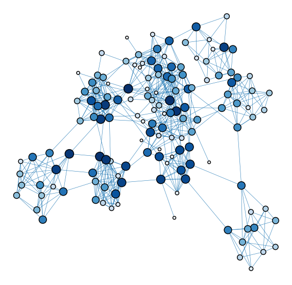
plot_network_color_scaled("gm_rank_order")
<AxesSubplot:xlabel='x', ylabel='y'>
Question
Graph matching requires an initialization. This could be an initial permutation. What would a good choice of initialization be?
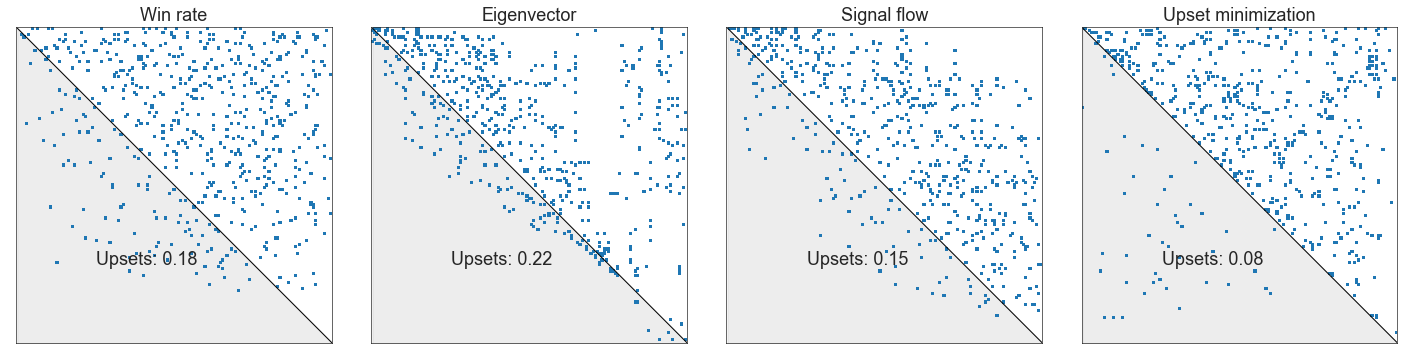
Compare these ranking schemes#
wr_perm_inds = np.argsort(-win_rates)

evec_perm_inds = np.argsort(-principal_evec)

sf_perm_inds = np.argsort(-z)

fig, axs = plt.subplots(1, 4, figsize=(20, 5))
plot_sorted_adjacency(adj, perm_inds=wr_perm_inds, ax=axs[0], title="Win rate")
plot_sorted_adjacency(adj, perm_inds=evec_perm_inds, ax=axs[1], title="Eigenvector")
plot_sorted_adjacency(adj, perm_inds=sf_perm_inds, ax=axs[2], title="Signal flow")
plot_sorted_adjacency(
    adj, perm_inds=gm_perm_inds, ax=axs[3], title="Upset minimization"
)
plt.tight_layout()
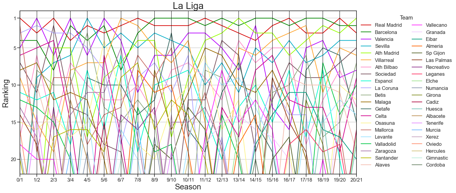
Ranking soccer teams#
from pathlib import Path

league = "LALIGA1"
data_dir = Path("./networks-course/data/sports/soccer")
start_year = 0
seasons = []
for year in range(start_year, 21):
    filename = f"{league}_{year}_{year+1}.csv"
    season_df = pd.read_csv(
        data_dir / filename, engine="python", usecols=[0, 1, 2, 3, 4, 5, 6, 7, 8]
    )
    season_df["season"] = f"{year}/{year+1}"
    seasons.append(season_df)
games = pd.concat(seasons, ignore_index=True)

edges = []
games["source"] = "none"
games["target"] = "none"
for idx, row in games.iterrows():
    if row["FTHG"] > row["FTAG"]:
        source = row["HomeTeam"]
        target = row["AwayTeam"]
        weight = 1
    elif row["FTHG"] < row["FTAG"]:
        target = row["HomeTeam"]
        source = row["AwayTeam"]
        weight = 1
    else:
        target = row["HomeTeam"]
        source = row["AwayTeam"]
        weight = 1 / 2
        edges.append(
            {
                "source": source,
                "target": target,
                "season": row["season"],
                "weight": weight,
            }
        )
        source = row["HomeTeam"]
        target = row["AwayTeam"]
        weight = 1 / 2
    # ignore ties for now
    edges.append(
        {"source": source, "target": target, "season": row["season"], "weight": weight}
    )
edgelist = pd.DataFrame(edges)

nodelist = list(edgelist["source"].unique()) + list(edgelist["target"].unique())
nodelist = np.unique(nodelist)
from graspologic.utils import remove_loops


def signal_flow(A):
    """Implementation of the signal flow metric from Varshney et al 2011

    Parameters
    ----------
    A : [type]
        [description]

    Returns
    -------
    [type]
        [description]
    """
    A = A.copy()
    A = remove_loops(A)
    W = (A + A.T) / 2

    D = np.diag(np.sum(W, axis=1))

    L = D - W

    b = np.sum(W * np.sign(A - A.T), axis=1)
    L_pinv = np.linalg.pinv(L)
    z = L_pinv @ b

    return z


def rank_signal_flow(A):
    sf = signal_flow(A)
    perm_inds = np.argsort(-sf)
    return perm_inds


def rank_graph_match_flow(A, n_init=100, max_iter=50, eps=1e-5, **kwargs):
    n = len(A)
    initial_perm = rank_signal_flow(A)
    init = np.eye(n)[initial_perm]
    match_mat = np.zeros((n, n))
    triu_inds = np.triu_indices(n, k=1)
    match_mat[triu_inds] = 1
    gm = GraphMatch(
        n_init=n_init, max_iter=max_iter, init="barycenter", eps=eps, **kwargs
    )
    perm_inds = gm.fit_predict(match_mat, A)
    return perm_inds


def calculate_p_upper(A):
    A = remove_loops(A)
    n = len(A)
    triu_inds = np.triu_indices(n, k=1)
    upper_triu_sum = A[triu_inds].sum()
    total_sum = A.sum()
    upper_triu_p = upper_triu_sum / total_sum
    return upper_triu_p
rankings = []
ranking_stats = []
for season, season_edges in edgelist.groupby("season", sort=False):
    g = nx.from_pandas_edgelist(
        season_edges, edge_attr="weight", create_using=nx.MultiDiGraph
    )
    season_nodes = np.intersect1d(nodelist, g.nodes)
    adj = nx.to_numpy_array(g, nodelist=season_nodes)
    perm_inds = rank_graph_match_flow(adj, n_init=50)
    p_upper = calculate_p_upper(adj[np.ix_(perm_inds, perm_inds)])
    rankings.append(
        pd.Series(
            data=np.arange(len(season_nodes)),
            name=season,
            index=season_nodes[perm_inds],
        )
    )
    ranking_stats.append(
        {
            "p_upper": p_upper,
            "season": season,
            "season_start": int(season.split("/")[0]),
        }
    )
ranking_stats = pd.DataFrame(ranking_stats)
rankings = pd.DataFrame(rankings).T
rankings.index.name = "team"
rankings["mean"] = rankings.fillna(30).mean(axis=1)
rankings = rankings.sort_values("mean")
times_not_in_league = rankings.isna().sum(axis=1)
common_teams = rankings.index[times_not_in_league < 5]
import colorcet as cc
plot_rankings = rankings.fillna(30).reset_index().drop("mean", axis=1)
fig, ax = plt.subplots(1, 1, figsize=(20, 10))
pd.plotting.parallel_coordinates(
plot_rankings,
class_column="team",
ax=ax,
color=cc.glasbey_light,
)
ax.get_legend().remove()
ax.set(ylim=(21, -1))
ax.legend(bbox_to_anchor=(1, 1), loc="upper left", ncol=2, title="Team")
ticks = np.array([1, 5, 10, 15, 20])
ax.set(yticks=ticks - 1, yticklabels=ticks)
ax.set_title("La Liga", fontsize="xx-large")
ax.set_xlabel("Season", fontsize="x-large")
ax.set_ylabel("Ranking", fontsize="x-large")
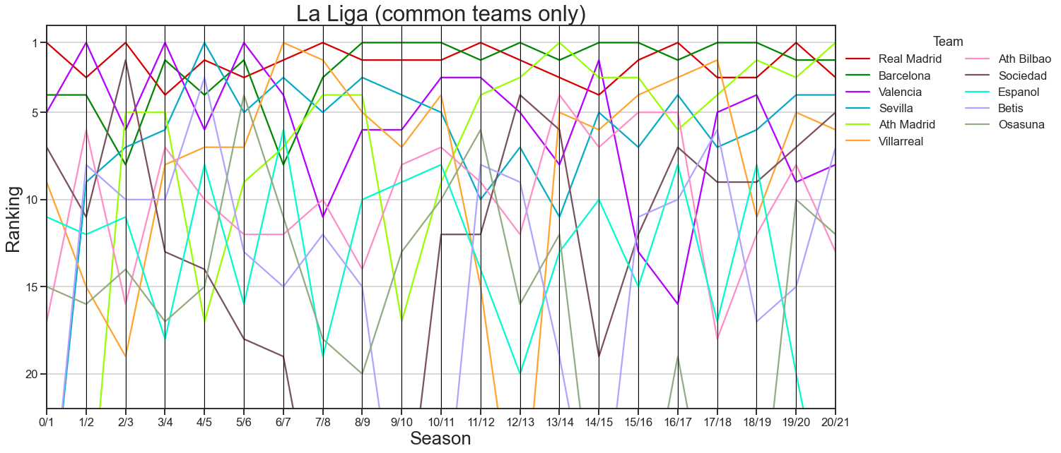
# plot only the teams that are usually in la liga
plot_rankings = plot_rankings[plot_rankings["team"].isin(common_teams)]
fig, ax = plt.subplots(1, 1, figsize=(20, 10))
pd.plotting.parallel_coordinates(
plot_rankings,
class_column="team",
ax=ax,
color=cc.glasbey_light,
)
ax.get_legend().remove()
ax.set(ylim=(21, -1))
ax.legend(bbox_to_anchor=(1, 1), loc="upper left", ncol=2, title="Team")
ticks = np.array([1, 5, 10, 15, 20])
ax.set(yticks=ticks - 1, yticklabels=ticks)
ax.set_title("La Liga (common teams only)", fontsize="xx-large")
ax.set_xlabel("Season", fontsize="x-large")
ax.set_ylabel("Ranking", fontsize="x-large")
Text(0, 0.5, 'Ranking')
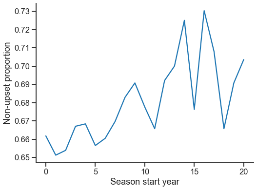
fig, ax = plt.subplots(1, 1, figsize=(8, 6))
sns.lineplot(data=ranking_stats, x="season_start", y="p_upper")
ticks = [0, 5, 10, 15, 20]
_ = ax.set(
    xticks=ticks,
    xticklabels=ticks,
    xlabel="Season start year",
    ylabel="Non-upset proportion",
)
ax.spines[["top", "right"]].set_visible(False)
Other applications#
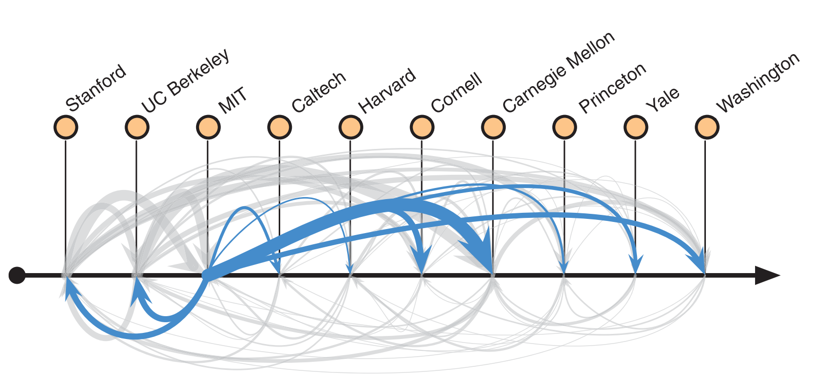
Fig. 24 Ranking of a network of faculty hires in computer science. Figure from Clauset et al. [2].#
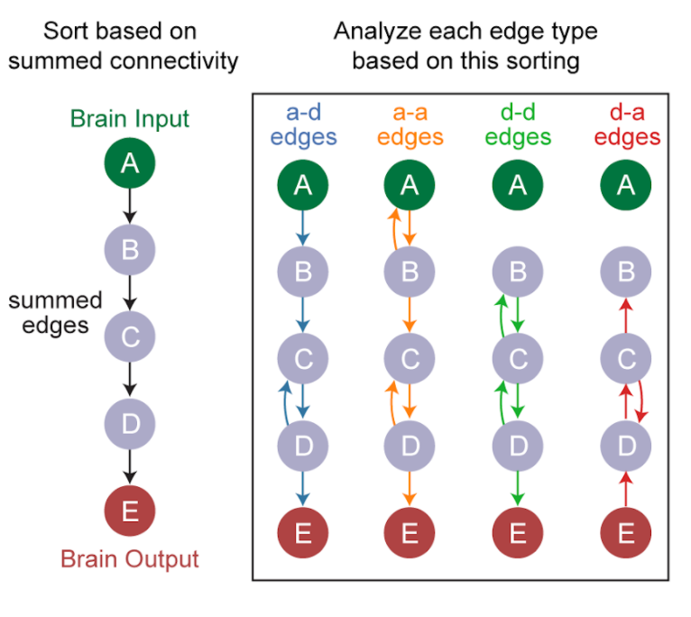
Fig. 25 Ordering the predominant direction of flow in a network of neurons, and comparing between edge types. Figure by Michael Winding.#