Community detection#
Community detection is the process of dividing a network into communities, where each community is some subset of nodes which connect more within community than without. This is an old and famous network science problem. It has applications across a wide range of disciplines. To name a just a few:
Predicting “workgroups” in organizational communication networks [2]
Grouping researchers into fields based on networks of collaboration [3]
Clustering networks formed by nearest neighbors in high-dimensional data
Much of the discussion/derivation in this notebook is based on Sections 7.7 and 14.2 from Mark Newman’s “Networks” [1].
Modularity#
From Wikipedia, in general usage, “modularity is the degree to which a system’s components may be separated and recombined.” The definition in network science is similar in spirit but has a more specific meaning. In words, modularity it is “the strength of division of a network into modules (also called groups, clusters or communities). Networks with high modularity have dense connections between the nodes within modules but sparse connections between nodes in different modules.”
How do we write this down mathematically? To begin, lets consider an undirected, unweighted network with no loops, with \(n \times n\) adjacency matrix \(A\).
As usual, we’ll let \(k\) be an \(n\)-length vector with the degree of each node. \(m\) will be the total number of edges.
First, we’d like some way of measuring the strength of edges within groups. Let \(\delta(\tau_i, \tau_j)\) be an indicator function which is 1 if \(i\) and \(j\) are in the same group, and 0 otherwise. Then, the total number of within-community edges is:
Note that we include the factor of \(\frac{1}{2}\) because otherwise edges would be counted twice in the sum.
Now, we want to optimize some function of the expression above, but note that as written, we could trivially put all nodes in the same group and that would maximize the expression we have written. So, we are going to add a term that will balance how many edges are within a group by how many edges we’d expect within a group based on a random model.
Specifically, we’ll use the random model where each node has its observed degree (\(k_i\)), but edges are arranged at random. How many edges are expected between nodes under this model?
Consider node \(i\) for the moment, and lets compute the probability of a particular edge \((i,j)\). Let’s select one of the edges attached to \(i\). Note that there are \(2m-1\) remaining edge stubs (sometimes called half edges) in the network. If the wiring is random, then the probability of connecting to any other edge stub is the same. Therefore, the probability of connecting to node \(j\) is proportional to the degree of that node: \(\frac{k_j}{2m-1}\). This is the probability of the original half-edge we chose being connected to \(j\), but any half-edge connected to \(i\) could have made the edge \((i, j)\). And how many of these half-edges are there? \(k_i\) of them. Therefore, the overall probability that \(i\) is connected to \(j\) is \(\frac{k_i k_j}{2m-1}\). Usually since \(m\) is so large for most networks, we drop the \(-1\) and consider
Note
In the logic above, we omit some details about multiple edges between the same pair of nodes under this random model, and the possibility of loops. Like the issue of \(2m\) vs. \(2m-1\), these details are negligible as the number of edges/nodes get large, so we ignore them for simplicity.
Great, this is roughly the probability of the edge \((i, j)\), but recall that we were interested in something like “given a partition \(\tau\) of my network, how many edges should I expect to be within-group under this silly null model?”. Using the same logic as before, we can compute this expected value by summing over this expected probability matrix.
Going back to our original expression, we literally take the difference of the observed number of edges that are within-group minus the number we’d expect by chance.
Lastly, it is usually more interpretable to make this quantity a proportion of edge rather than a count, so we divide by \(m\). Thus, we arrive at the expression usually defined as modularity.
Note
People often talk about “the modularity of this network” as if it is a function of the adjacency matrix only: \(Q(A)\). Note that modularity is absolutely a function of a network \(A\) AND a partition, \(\tau\).
Naive optimization#
Thus far, we’ve talked about how we can compute this modularity quantity for a given \(A\) and partition \(\tau\). But remember, we are talking about community detection! In other words, we’re trying to infer \(\tau\) from the data.
For the next few explanations, we are going to restrict ourselves to the case where we are only seeking to divide a network into two communities since it will make the explanations easier, but note that everything still works for more communities.
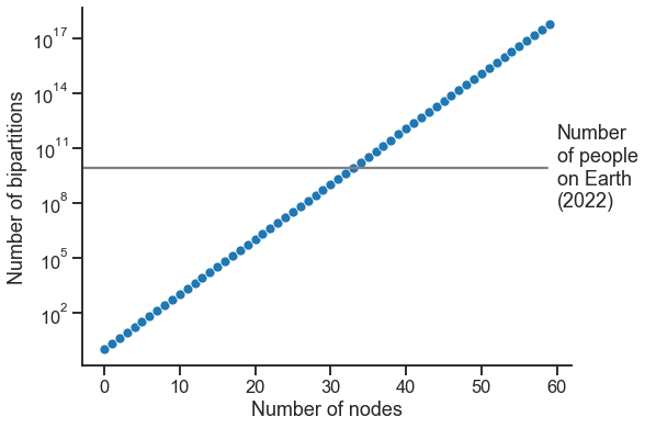
Question
Let’s say you have \(n\) nodes, and you’re only considering community detection into two groups. How many different partitions, \(\tau\), are there?
import numpy as np

ns = np.arange(60)

n_possible_taus = 2**ns

import matplotlib.pyplot as plt
import seaborn as sns

sns.set_context("talk")

fig, ax = plt.subplots(1, 1, figsize=(8, 6))
sns.scatterplot(x=ns, y=n_possible_taus, ax=ax)
ax.set_yscale("log")
ax.set(xlabel="Number of nodes", ylabel="Number of bipartitions")
world_pop = 8_000_000_000
ax.axhline(world_pop, xmax=0.95, color="grey")
ax.text(60, world_pop, "Number\nof people\non Earth\n(2022)", va="center", ha="left")

ax.spines.right.set_visible(False)
ax.spines.top.set_visible(False)
Question
Let’s say you have a network \(A\), and I give you a random partition, \(\tau\). What is the silliest, most naive way you can think of trying to improve the modularity score?
For the next few examples, we’ll use the “polbooks” dataset, available at Netzschleuder. Each node is a book, and the nodes are linked by edges which represent “frequent copurchasing of those books by the same buyers” on Amazon.
import networkx as nx
import pandas as pd

g = nx.read_edgelist("networks-course/data/polbooks.csv/edges.csv", delimiter=",")

nodelist = list(g.nodes)
node_df = pd.DataFrame(index=nodelist)

pos = nx.kamada_kawai_layout(g)

xs = []
ys = []
for node in nodelist:
    xs.append(pos[node][0])
    ys.append(pos[node][1])
xs = np.array(xs)
ys = np.array(ys)

node_df["x"] = xs
node_df["y"] = ys

adj = nx.to_numpy_array(g, nodelist=nodelist)
n = adj.shape[0]

node_df["degree"] = adj.sum(axis=0)
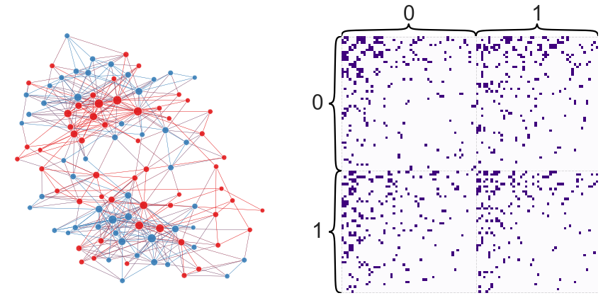
We’ll start by generating a random \(\tau\) with two communities.
# random bernoullis
rng = np.random.default_rng(888)
partition = rng.binomial(1, 0.5, size=n)

partition
array([0, 0, 0, 0, 1, 1, 1, 0, 0, 0, 1, 0, 0, 0, 1, 1, 1, 0, 0, 1, 0, 1,
       1, 1, 0, 0, 0, 0, 0, 0, 0, 0, 0, 1, 1, 1, 0, 1, 0, 1, 0, 1, 1, 0,
       1, 1, 0, 1, 0, 1, 0, 0, 1, 1, 1, 0, 1, 0, 0, 0, 1, 0, 0, 1, 0, 1,
       0, 0, 1, 0, 1, 1, 1, 0, 1, 1, 1, 0, 1, 0, 1, 0, 1, 1, 1, 0, 1, 0,
       0, 1, 1, 0, 1, 1, 0, 0, 1, 1, 1, 0, 1, 0, 0, 0, 0])
Clearly this random partition of our network is not very good:
def modularity_from_adjacency(sym_adj, partition, resolution=1):
    if isinstance(partition, dict):
        partition_labels = np.vectorize(partition.__getitem__)(
            np.arange(sym_adj.shape[0])
        )
    else:
        partition_labels = partition
    partition_labels = np.array(partition_labels)
    in_comm_mask = partition_labels[:, None] == partition_labels[None, :]
    degrees = np.squeeze(np.asarray(sym_adj.sum(axis=0)))
    degree_prod_mat = np.outer(degrees, degrees) / sym_adj.sum()
    mod_mat = sym_adj - resolution * degree_prod_mat
    return mod_mat[in_comm_mask].sum() / sym_adj.sum()


mod_score = modularity_from_adjacency(adj, partition)
mod_score
-0.014078496099876065
What would this partition look like plotted on our network?
from graspologic.plot import networkplot, heatmap

node_df["random_partition"] = partition


def plot_network_partition(adj, node_data, partition_key):
    fig, axs = plt.subplots(1, 2, figsize=(15, 7))

    networkplot(
        adj,
        x="x",
        y="y",
        node_data=node_data.reset_index(),
        node_alpha=0.9,
        edge_alpha=0.7,
        edge_linewidth=0.4,
        node_hue=partition_key,
        node_size="degree",
        edge_hue="source",
        ax=axs[0],
    )
    _ = axs[0].axis("off")

    _ = heatmap(
        adj,
        inner_hier_labels=node_data[partition_key],
        ax=axs[1],
        cbar=False,
        cmap="Purples",
        vmin=0,
        center=None,
        sort_nodes=True,
    )

    return fig, ax


plot_network_partition(adj, node_df, "random_partition")
(<Figure size 1080x504 with 4 Axes>,
 <AxesSubplot:xlabel='Number of nodes', ylabel='Number of bipartitions'>)
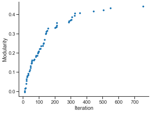
Next we’ll try a very simple algorithm for maximizing modularity. Starting from some initial partition \(\tau_0\), we proceed by simply picking a node at random, and then check whether switching the group assigned to that node increases the modularity. If it does, we move that node into that group. Otherwise, we revert it back to its original group label, and proceed to the next iteration of checking another random node’s label.
n_trials = 1000

best_scores = []
best_iterations = []
last_mod_score = mod_score
for iteration in range(n_trials):
    # choose a random node to perturb
    index = rng.choice(n)

    # check what group it is currently in, and swap it
    current_group = partition[index]
    if current_group:
        partition[index] = 0
    else:
        partition[index] = 1

    # compute modularity with this slightly modified partition
    mod_score = modularity_from_adjacency(adj, partition)

    # decide whether to keep that change or not
    if mod_score < last_mod_score:
        # swap it back
        if current_group:
            partition[index] = 1
        else:
            partition[index] = 0
    else:
        last_mod_score = mod_score
        best_scores.append(mod_score)
        best_iterations.append(iteration)

mod_score
0.4405468914701179
partition
array([0, 0, 0, 0, 0, 0, 0, 0, 0, 0, 0, 0, 0, 0, 0, 0, 0, 0, 0, 0, 0, 0,
       0, 0, 0, 0, 0, 0, 1, 0, 1, 1, 0, 0, 0, 0, 0, 0, 0, 0, 0, 0, 0, 0,
       0, 0, 0, 0, 0, 0, 0, 0, 0, 0, 0, 0, 0, 0, 0, 1, 1, 1, 1, 1, 0, 0,
       1, 0, 0, 0, 1, 1, 1, 1, 1, 1, 1, 1, 1, 1, 1, 1, 1, 1, 1, 0, 1, 1,
       1, 1, 1, 1, 1, 1, 1, 1, 1, 1, 1, 1, 1, 1, 1, 0, 0])
Below, we look at how modularity changes as this simple algorithm progresses through its iterations.
fig, ax = plt.subplots(1, 1, figsize=(8, 6))
sns.scatterplot(x=best_iterations, y=best_scores, ax=ax, s=40, linewidth=0)
ax.set(ylabel="Modularity", xlabel="Iteration")
ax.spines.right.set_visible(False)
ax.spines.top.set_visible(False)
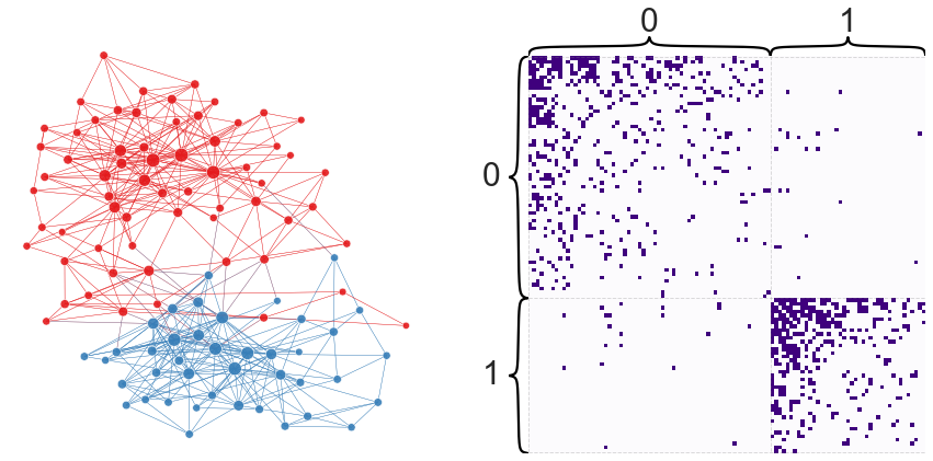
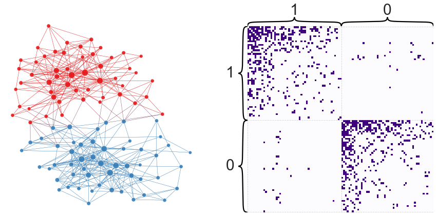
Let’s look at the partition we find when plotted over the network.
node_df["naive_partition"] = partition

plot_network_partition(adj, node_df, "naive_partition")
(<Figure size 1080x504 with 4 Axes>,
 <AxesSubplot:xlabel='Iteration', ylabel='Modularity'>)
Spectral optimization#
Next, we’ll look at one less silly way of optimizing modularity.
We can define the matrix \(B\), often called the modularity matrix as
Sticking to the case of two groups, let’s change our convention for \(\tau\) so that \(\tau_i = 1\) if node \(i\) is in group 1, and \(\tau_i = -1\) if it is in group 2.
Then, note that our indicator function has a nice expression now:
Now we can easily write our modularity function.
In matrix/vector form, we can write this as
Note that \(B\) is still a symmetric matrix (since we were concerned with undirected graphs).
from graspologic.utils import is_symmetric

B = nx.modularity_matrix(g, nodelist=nodelist)

is_symmetric(B)
True
Next, we proceed by making an approximation. We have a discrete optimization problem:
This is a difficult problem because of how many possible \(\tau\)s there are as we saw before, and the discrete nature of the problem. Note that \(\| \tau \|_2\), the Euclidean norm of \(\tau\), will always be \(\sqrt{n}\). We relax our problem so that \(\tau\) does not have to be discrete, but keeps its length.
This problem has the same solution (ignoring constants that don’t affect the result besides scaling):
Note that this expression is what’s known as a Rayleigh-Ritz ratio or Rayleigh quotient. We won’t go into deriving the properties of this, but note that if you know what an eigendecomposition is, it is not to difficult to work out the following property: for a symmetric matrix \(B\) in the expression above, \(R(B, \tau) \in [\lambda_{min}, \lambda_{max}]\) where \(\lambda_{min}\) and \(\lambda_{max}\) are the smallest and largest eigenvalues of \(B\), respectively.
So, this tells us that the maximum is achieved when \(R(B, \tau) = \lambda_{max}\). And how can we achieve this upper bound? By setting \(\tau\) to be the eigenvector corresponding to the largest eigenvalue (call this \(x\)):
However, now we need to get back to our discrete optimization problem by projecting back onto the discrete solutions, e.g. where \(\tau\) is only \(-1\) or \(1\). To do so, we maximize the inner products between this discrete solution, \(\tau\), and our eigenvector \(x\):
To do so, we want \(x_i \tau_i\) to be positive for all \(i\). We can achieve this by setting
Thus, our simple algorithm is now to:
Compute the eigenvector corresponding to the largest eigenvalue of \(B\), and
Threshold the corresponding eigenvector based on its sign to get our partition.
Note
Be careful about assuming the order in which eigenvalues/eigenvectors are returned.
Here, they are returned in decreasing order by the eigh function, which is faster
for symmetric (Hermitian) matrices.
eigenvalues, eigenvectors = np.linalg.eigh(B)
first_eigenvector = np.squeeze(np.asarray(eigenvectors[:, -1]))
first_eigenvector
array([-0.02550912, -0.02456848, -0.00170053, -0.19262125,  0.01632424,
       -0.02333085, -0.05243838,  0.01705257, -0.23826617, -0.14694971,
       -0.13066785, -0.17909148, -0.2278586 , -0.13652453, -0.09609015,
       -0.0537466 , -0.03258368, -0.07848085, -0.04078242, -0.02814099,
       -0.09584042, -0.07332282, -0.07773025, -0.11014213, -0.11975091,
       -0.05089722, -0.11127976, -0.12026225,  0.03486849, -0.03053454,
        0.18966993,  0.10967268, -0.07009965, -0.10030317, -0.08262   ,
       -0.03008297, -0.0535839 , -0.07084867, -0.06221648, -0.0758389 ,
       -0.1696462 , -0.10436962, -0.07279506, -0.04798468, -0.07367568,
       -0.08792768, -0.05454009, -0.17501516, -0.0219253 ,  0.01486383,
       -0.02666456, -0.00957711, -0.01668981, -0.03091357, -0.07826915,
       -0.03811773, -0.02425889, -0.02312067,  0.01822838,  0.04866926,
        0.02113664,  0.0199537 ,  0.04687952,  0.01967049,  0.02755088,
        0.01022675,  0.19268054,  0.03578428,  0.01618876,  0.0036785 ,
        0.08375239,  0.13868297,  0.2027985 ,  0.21677572,  0.18442602,
        0.17949498,  0.14169565,  0.06326878,  0.06912215,  0.11280441,
        0.0614348 ,  0.04966937,  0.13492524,  0.10857716,  0.22677681,
        0.03713454,  0.14403887,  0.06610225,  0.07608982,  0.08987874,
        0.05797735,  0.08678585,  0.05088125,  0.07853913,  0.05733061,
        0.02542713,  0.07555278,  0.07673903,  0.0571795 ,  0.1187217 ,
        0.12131853,  0.04811651,  0.00866984,  0.00311235,  0.00329647])
eig_partition = first_eigenvector.copy()
eig_partition[eig_partition > 0] = 1
eig_partition[eig_partition <= 0] = 0
eig_partition = eig_partition.astype(int)
eig_partition
array([0, 0, 0, 0, 1, 0, 0, 1, 0, 0, 0, 0, 0, 0, 0, 0, 0, 0, 0, 0, 0, 0,
       0, 0, 0, 0, 0, 0, 1, 0, 1, 1, 0, 0, 0, 0, 0, 0, 0, 0, 0, 0, 0, 0,
       0, 0, 0, 0, 0, 1, 0, 0, 0, 0, 0, 0, 0, 0, 1, 1, 1, 1, 1, 1, 1, 1,
       1, 1, 1, 1, 1, 1, 1, 1, 1, 1, 1, 1, 1, 1, 1, 1, 1, 1, 1, 1, 1, 1,
       1, 1, 1, 1, 1, 1, 1, 1, 1, 1, 1, 1, 1, 1, 1, 1, 1])
How does this partition compare to our earlier one?
modularity_from_adjacency(adj, partition)
0.44240825581933463
node_df["eig_partition"] = eig_partition

plot_network_partition(adj, node_df, "eig_partition")
(<Figure size 1080x504 with 4 Axes>,
 <AxesSubplot:xlabel='Iteration', ylabel='Modularity'>)
Agglomerative optimization - Louvain/Leiden#
We won’t get into as much detail about more complicated methods for optimizing the modularity, but I wanted to mention these algorithms since they are somewhat state-of-the-art.
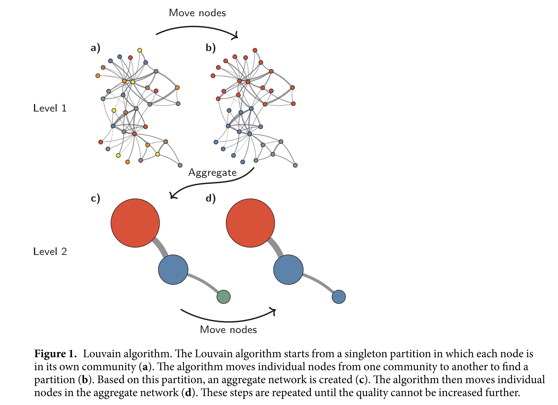
Fig. 6 High-level summary of the Louvain algorithm [4]. Figure from the Leiden paper [5], which further improved the Louvain algorithm.#
The Leiden algorithm scales to very large networks, and usually provides competitive
modularity scores. It is easy to use from graspologic.
from graspologic.partition import leiden, modularity

leiden_partition_map = leiden(g, random_seed=7)
type(leiden_partition_map)
dict
# this is necessary just because this modularity implementation assumes a weighted graph
nx.set_edge_attributes(g, 1, "weight")

modularity(g, leiden_partition_map)
0.5264061784955857
Note that this algorithm (like most) is not deterministic.
leiden_partition_map = leiden(g, random_seed=6)
modularity(g, leiden_partition_map)
0.5266195669499848
Often, it’s a good idea to take the best over multiple runs of the algorithm.
leiden_partition_map = leiden(g, trials=100)
modularity(g, leiden_partition_map)
0.5270746242563541
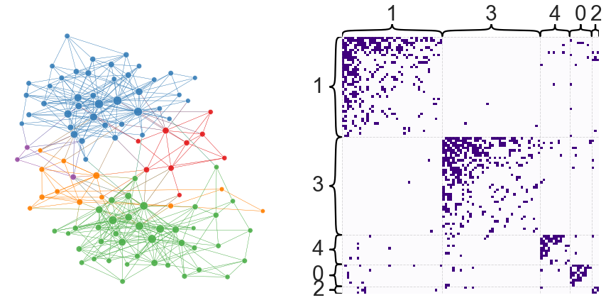
node_df["leiden_partition"] = node_df.index.map(leiden_partition_map)

plot_network_partition(adj, node_df, "leiden_partition")
(<Figure size 1080x504 with 4 Axes>,
 <AxesSubplot:xlabel='Iteration', ylabel='Modularity'>)
Know what modularity gives you#
I briefly want to mention one point of confusion I’ve seen, in particular when thinking about stochastic block models (SBM) and community detection.
I always refer to community detection to mean “finding assortative or homophillic groups of nodes.” Both of these terms just mean “like connects to like.” Conversely, other algorithms might be able to find disassortative groups of nodes, which I would not call communities.
Let’s see how community detection performs in both of these cases.
from graspologic.simulations import sbm

B_assort = np.array([[0.9, 0.1], [0.1, 0.8]])
B_disassort = np.array([[0.1, 0.9], [0.9, 0.05]])

A_assort, labels_assort = sbm([50, 50], B_assort, return_labels=True)
A_disassort, labels_disassort = sbm([50, 50], B_disassort, return_labels=True)

nodelist = np.arange(100)

partition_map_assort = leiden(A_assort, trials=10)
partition_map_disassort = leiden(A_disassort, trials=10)
partition_assort = np.vectorize(partition_map_assort.get)(nodelist)
partition_disassort = np.vectorize(partition_map_disassort.get)(nodelist)

fig, axs = plt.subplots(2, 2, figsize=(10, 10))

heatmap_kws = dict(cbar=False)

ax = axs[0, 0]
heatmap(A_assort, inner_hier_labels=labels_assort, ax=ax, **heatmap_kws)
ax.set_ylabel("True partition", labelpad=40)
ax.set_title("Assortative SBM", pad=50)

ax = axs[0, 1]
heatmap(A_disassort, inner_hier_labels=labels_disassort, ax=ax, **heatmap_kws)
ax.set_title("Disassortative SBM", pad=50)

ax = axs[1, 0]
heatmap(A_assort, inner_hier_labels=partition_assort, ax=ax, **heatmap_kws)
ax.set_ylabel("Estimated partition", labelpad=40)

ax = axs[1, 1]
_ = heatmap(A_disassort, inner_hier_labels=partition_disassort, ax=ax, **heatmap_kws)
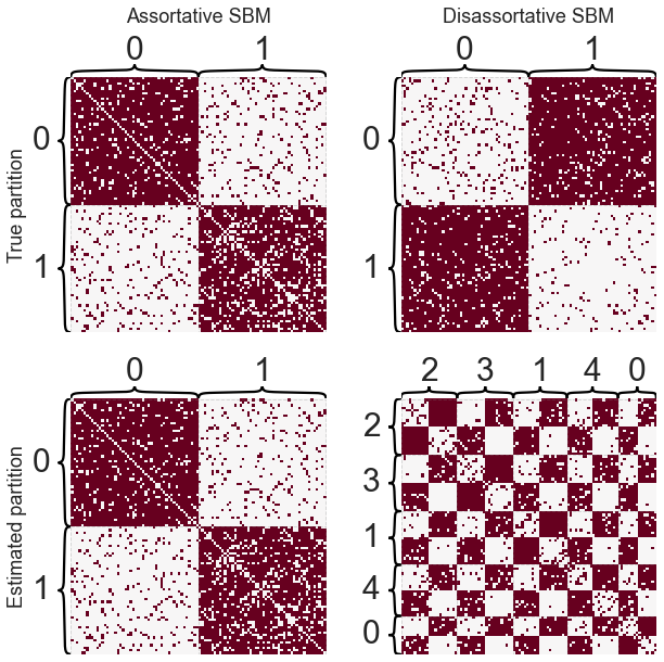
Note
Other families of algorithms would be able to find this disassortative partition - it’s just not what modularity is looking for.
Issues with modularity maximization#
Resolution limit#
While these algorithms are very useful, they have problems. The first is called the resolution limit. This idea is basically that for a large network, small communities (even if very clear) can be impossible to detect for any modularity maximization algorithm. There is further discussion of this issue in Section 14.2.6 of Newman’s Networks book.
Overfitting#
Modularity maximization algorithms can also have the converse problem, that is, finding community structure when it is not present. This is best demonstrated by example.
from graspologic.simulations import er_np

n_nodes = 100

A_er = er_np(n_nodes, 0.1)

leiden_partition_map = leiden(A_er)

nodes = np.arange(n_nodes)
partition_labels = np.vectorize(leiden_partition_map.get)(nodes)

_ = heatmap(A_er, inner_hier_labels=partition_labels, cbar=False)
Even for this very simple, completely random (Erdos-Renyi) network, Leiden found several communities - further, these communities do look more densely connected within. However, the key point here is that these “communities” arose completely by chance even with the simplest null model.
Alternatives to modularity#
While we haven’t had time to discuss them, there are many alternatives to modularity maximization for finding communities. For instance:
InfoMap#
InfoMap uses random walks and an information theory framework. The idea is that good communities should allow you to easily compress the amount of information that would be required to encode the path of a random walker.

Fig. 7 Illustration of the idea of encoding the path of random walkers used by InfoMap. Figure from Emmons and Mucha [6].#
Statistical inference (SBM + similar)#
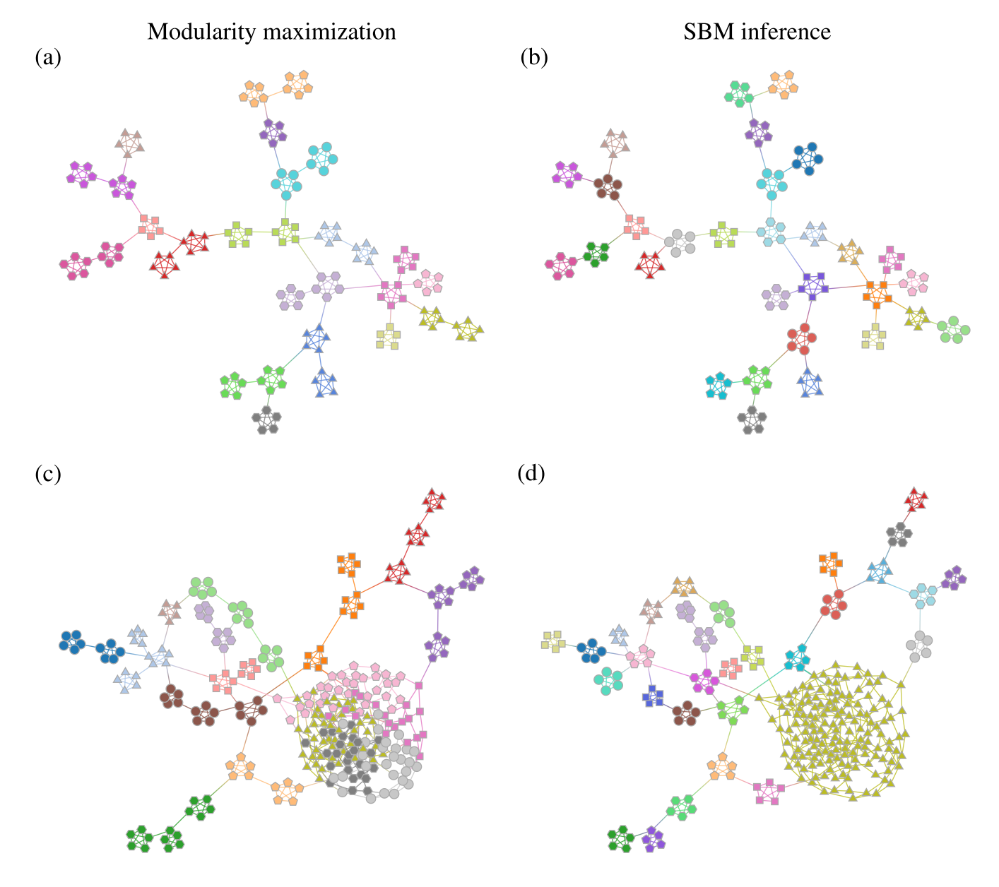
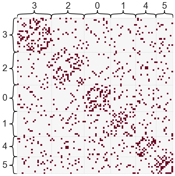
Fig. 8 Demonstration of how inferring a statistical model (like an assortative SBM) can alleviate some of the issues from modularity maximization. Figure from Peixoto [7].#
Other code#
CDlib has a wide range of community detection algorithms.
NetworkX’s community section has a few algorithms.
graph-tool has some new tools for assortative community detection based on statistical models.
References#
Mark Newman. Networks. Oxford university press, 2018.
Tiona Zuzul, Emily Cox Pahnke, Jonathan Larson, Patrick Bourke, Nicholas Caurvina, Neha Parikh Shah, Fereshteh Amini, Youngser Park, Joshua Vogelstein, Jeffrey Weston, and others. Dynamic silos: increased modularity in intra-organizational communication networks during the covid-19 pandemic. arXiv preprint arXiv:2104.00641, 2021.
Michelle Girvan and Mark EJ Newman. Community structure in social and biological networks. Proceedings of the national academy of sciences, 99(12):7821–7826, 2002.
Vincent D Blondel, Jean-Loup Guillaume, Renaud Lambiotte, and Etienne Lefebvre. Fast unfolding of communities in large networks. Journal of statistical mechanics: theory and experiment, 2008(10):P10008, 2008.
Vincent A Traag, Ludo Waltman, and Nees Jan Van Eck. From louvain to leiden: guaranteeing well-connected communities. Scientific reports, 9(1):1–12, 2019.
Scott Emmons and Peter J Mucha. Map equation with metadata: varying the role of attributes in community detection. Physical Review E, 100(2):022301, 2019.
Tiago P Peixoto. Descriptive vs. inferential community detection: pitfalls, myths and half-truths. arXiv preprint arXiv:2112.00183, 2021.