Graph matching

Some of this lesson is taken directly from the graspologic tutorials on graph matching, mostly written by Ali Saad-Eldin with help from myself.

Why match graphs?

Graph matching comes up in a ton of different contexts!

• Computer vision: comparing objects

• Communication networks:

  • Finding noisy subgraphs

  • Matching different social networks

• Neuroscience: finding the same nodes on different sides of a brain

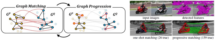
Fig. 15 Application of graph matching in computer vision. Figure from here.

Fig. 16 Potential application of graph matching in a communication subnetwork. Figure from The Wire, Season 3, Episode 7.

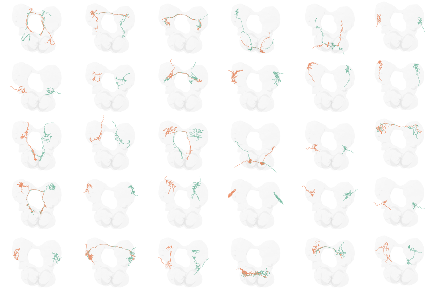
Fig. 17 Application of graph matching to predict homologous neurons in a brain connectome.

Permutations

To start to understand graph matching, we first need to understand permutations and permutation matrices.

A permutation can be thought of as a specific ordering or arrangement of some number of objects.

Question

How many permutations are there of \(n\) objects?

Permutations, for us, will be represented by permutation matrices. A permutation matrix is \(n \times n\), with all zeros except for \(n\) 1s. More specifically, each row and column has exactly one 1 in it. Let’s look at what a permutation matrix times a vector looks like.

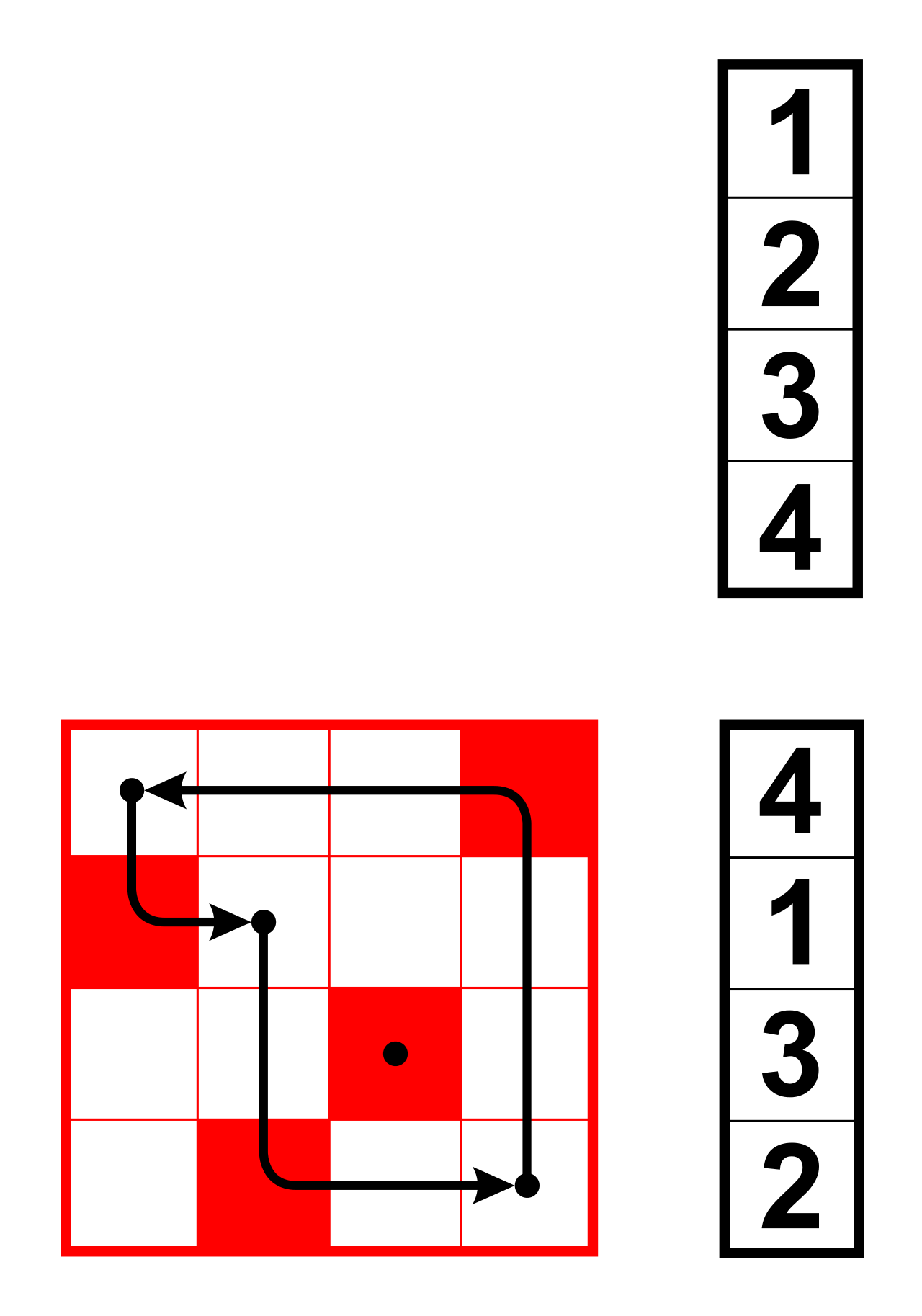
Fig. 18 A permutation matrix multiplied by a vector. The red elements of the matrix indicate the 1s. Image from Wikipedia.

So, we see that if we look at the permutation matrix, the row index represents the index of the new position of object \(i\). The column index represents the original position of an object. So, if we have a 1 at position \((1, 4)\), that means the first object was the fourth object in the original arangement.

Note that this also works for matrices: each column of a matrix \(A\) would be permuted the same way as the vector in the example above. So, we can think of

\[PA\]

as permuting the rows of the matrix \(A\).

Note that post-multiplication by the matrix \(P\) works the opposite way (try it out yourself if you don’t see this, or refer to the Wikipedia article). For this reason, if we wanted to permute the columns of \(A\) in the same way, we’d have to do

\[AP^T\]

Question

How can we permute the rows and columns of the matrix \(A\) in the same way? Why do we care about this for networks?

Graph matching problem

Why do we care about permutations for the problem of graph matching? Graph matching refers to the problem of finding a mapping between the nodes of one graph (\(A\)) and the nodes of some other graph, \(B\). For now, consider the case where the two networks have exactly the same number of nodes. Then, this problem amounts to finding a permutation of the nodes of one network with regard to the nodes of the other. Mathematically, we can think of this as comparing \(A\) vs. \(P B P^T\).

Note

You can think of graph matching as a more general case of the graph isomorphism problem.

In the case of graph matching, we don’t assume that the graphs must be exactly the same when matched, while for the graph isomorphism problem, we do.

How can we measure the quality of this alignment between two networks, given what we’ve talked about so far? Like when we talked about approximating matrices in the embeddings section, one natural way to do this is via the Frobenius norm of the difference.

\[e(P) = \|A - PBP^T\|_F\]

Question

In words, what is this quantity \(e(P)\) measuring with respect to the edges of two unweighted networks?

We can use this same definition above for any type of network: unweighted or weighted, directed or undirected, with or without self-loops.

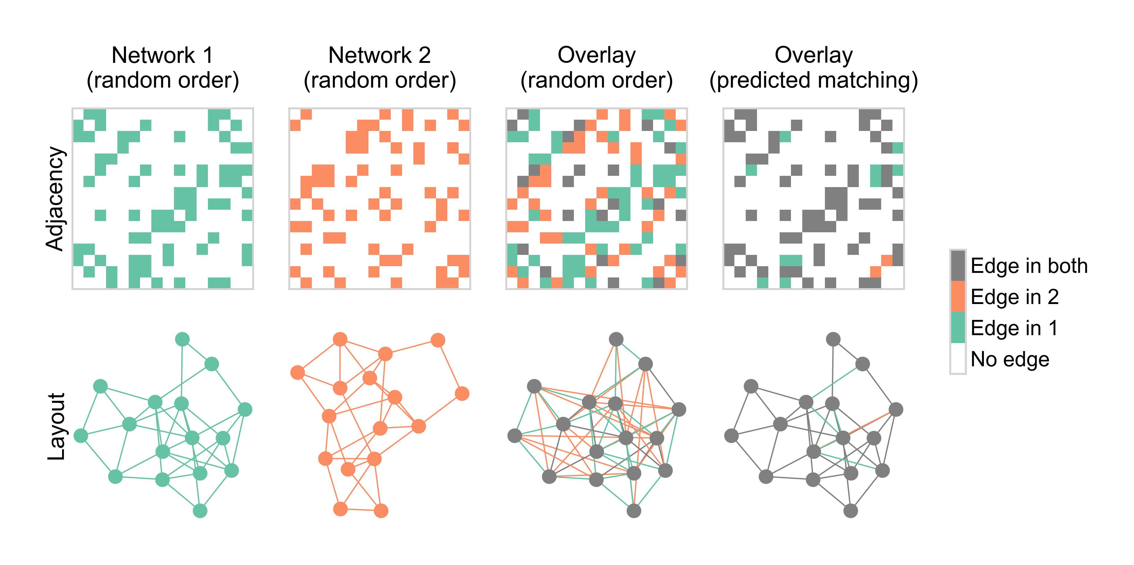
Fig. 19 Diagram explaining graph matching.

Solving the graph matching problem

Many solutions for the problem above have been proposed - note that all of these are approximate solutions, and they tend to scale fairly poorly (in the number of nodes) compared to some of the other algorithms we have discussed so far. Nevertheless, a lot of progress has been made. I’m just going to focus on one family of algorithms based on the work of Vogelstein et al. [2].

As we discussed when looking at the spectral method for maximizing modularity, we have a discrete problem, but we’d like to use continuous optimization tools where we can take gradients. To make this possible, the Fast Approximate Quadradic (FAQ) method first relaxes the constraint that \(P\) be a permutation matrix. Via the Birkhoff-von Neumann theorem, it can be shown that the convex hull of the permutation matrices is the set of doubly stochastic matrices. A doubly stochastic matrix just has row and columns sums equal to 1, but does not necessarily have to have all nonzero elements equal to 1. This theorem is just saying that if I take a weighted average of any two permutation matrices, the row and columns sums of the result must be 1.

It can be shown that minimizing our \(e(P)\) above is equivalent to

\[\min_P -\text{trace}(APB^T P^T)\]

Note

The quadratic assignment problem can be written as \(\min_P \text{trace}(APB^T P^T)\) - since these are just a sign flip away, any algorithm which solves one can be easily used to solve the other.

Calling our doubly stochastic matrices \(D\), we now have

\[\min_D -\text{trace}(ADB^T D^T)\]

Given this relaxation, we can now begin to take gradients in our space of matrices. I won’t go into every detail, but the algorithm we end up using is something like:

1. Start with some initial position - note that this position is a doubly stochastic matrix.

2. Compute the gradient of the expression above with respect to \(D\). This gives us our “step direction.”

3. Compute a step size (how far to go in that direction in the space of matrices) by searching over the line between our current position and the one computed in 2.

4. Update our position based on 3.

5. Repeat 2.-4. until some convergence criterion is reached.

6. Project back to the set of permutation matrices.

Graph matching with graspologic

Basic graph matching

Thankfully, all of this is implemented in graspologic. Let’s start by generating a random network (ER). We’ll then make a permuted copy of itself.

import numpy as np
from graspologic.match import graph_match
from graspologic.simulations import er_np

n = 50
p = 0.3

np.random.seed(1)
rng = np.random.default_rng(8888)

G1 = er_np(n=n, p=p)
node_shuffle_input = np.random.permutation(n)
G2 = G1[np.ix_(node_shuffle_input, node_shuffle_input)]
print("Number of edge disagreements: ", np.sum(abs(G1 - G2)))

import matplotlib.pyplot as plt
from graspologic.plot import heatmap

fig, axs = plt.subplots(1, 2, figsize=(10, 5))
heatmap(G1, cbar=False, title="G1 [ER-NP(50, 0.3) Simulation]", ax=axs[0])
_ = heatmap(G2, cbar=False, title="G2 [G1 Randomly Shuffled]", ax=axs[1])

Now, let’s solve the graph matching problem.

_, perm_inds, _, _ = graph_match(G1, G2, rng=rng)
G2 = G2[np.ix_(perm_inds, perm_inds)]
print("Number of edge disagreements: ", np.sum(abs(G1 - G2)))

So, we’ve exactly recovered the correct permutation - note that this won’t always be true.

Adding seed nodes

Next, we explore the use of “seed” nodes. Imagine you have two networks that you want to match, but you already know that a handful of these nodes are correctly paired. These nodes are called seeds, which you can incorporate into the optimization in graspologic via techniques described in Fishkind et al. [3].

For this example, we use a slightly different network model - we create two stochastic block models, but the edges are correlated so that the two networks are similar but not exactly the same.

import seaborn as sns
from graspologic.simulations import sbm_corr

sns.set_context("talk")

np.random.seed(8888)

directed = False
loops = False
n_per_block = 75
n_blocks = 3
block_members = np.array(n_blocks * [n_per_block])
n_verts = block_members.sum()
rho = 0.9
block_probs = np.array([[0.7, 0.3, 0.4], [0.3, 0.7, 0.3], [0.4, 0.3, 0.7]])
fig, ax = plt.subplots(1, 1, figsize=(4, 4))
sns.heatmap(block_probs, cbar=False, annot=True, square=True, cmap="Reds", ax=ax)
ax.set_title("SBM block probabilities")

A1, A2 = sbm_corr(block_members, block_probs, rho, directed=directed, loops=loops)
fig, axs = plt.subplots(1, 3, figsize=(10, 5))
heatmap(A1, ax=axs[0], cbar=False, title="Graph 1")
heatmap(A2, ax=axs[1], cbar=False, title="Graph 2")
_ = heatmap(A1 - A2, ax=axs[2], cbar=False, title="Diff (G1 - G2)")

Here we see that after shuffling the second graph, there are many more edge disagreements, as expected.

node_shuffle_input = np.random.permutation(n_verts)
A2_shuffle = A2[np.ix_(node_shuffle_input, node_shuffle_input)]
node_unshuffle_input = np.array(range(n_verts))
node_unshuffle_input[node_shuffle_input] = np.array(range(n_verts))

fig, axs = plt.subplots(1, 3, figsize=(10, 5))
heatmap(A1, ax=axs[0], cbar=False, title="Graph 1")
heatmap(A2_shuffle, ax=axs[1], cbar=False, title="Graph 2 shuffled")
_ = heatmap(A1 - A2_shuffle, ax=axs[2], cbar=False, title="Diff (G1 - G2 shuffled)")

First, we will run graph matching on graph 1 and the shuffled graph 2 with no seeds, and return the match ratio, that is the fraction of vertices that have been correctly matched.

perm_first, perm_inds, score, misc = graph_match(A1, A2_shuffle, rng=rng)
# these other 3 returns we often don't use, but they are there if you want them and
# are explained in the docs. for the most part, we care about "perm_inds" which tell us
# how to permute the second graph to match the first graph.

A2_unshuffle = A2_shuffle[np.ix_(perm_inds, perm_inds)]

fig, axs = plt.subplots(1, 3, figsize=(10, 5))
heatmap(A1, ax=axs[0], cbar=False, title="Graph 1")
heatmap(A2_unshuffle, ax=axs[1], cbar=False, title="Graph 2 unshuffled")
heatmap(A1 - A2_unshuffle, ax=axs[2], cbar=False, title="Diff (G1 - G2 unshuffled)")

match_ratio = 1 - (np.count_nonzero(abs(perm_inds - node_unshuffle_input)) / n_verts)
print("Match Ratio with no seeds: ", match_ratio)

While the predicted permutation for graph 2 did recover the basic structure of the stochastic block model (i.e. graph 1 and graph 2 look qualitatively similar), we see that the number of edge disagreements between them is still quite high, and the match ratio quite low.

Next, we will run SGM with 10 randomly selected seeds. Although 10 seeds is only about 4% of the 300 node graph, we will observe below how much more accurate the matching will be compared to having no seeds.

import random

seeds1 = np.sort(random.sample(list(range(n_verts)), 10))
seeds1 = seeds1.astype(int)
seeds2 = np.array(node_unshuffle_input[seeds1])
partial_match = np.column_stack((seeds1, seeds2))

_, perm_inds, _, _ = graph_match(A1, A2_shuffle, partial_match=partial_match, rng=rng)
A2_unshuffle = A2_shuffle[np.ix_(perm_inds, perm_inds)]

fig, axs = plt.subplots(1, 3, figsize=(10, 5))
heatmap(A1, ax=axs[0], cbar=False, title="Graph 1")
heatmap(A2_unshuffle, ax=axs[1], cbar=False, title="Graph 2 unshuffled")
heatmap(A1 - A2_unshuffle, ax=axs[2], cbar=False, title="Diff (G1 - G2 unshuffled)")

match_ratio = 1 - (np.count_nonzero(abs(perm_inds - node_unshuffle_input)) / n_verts)
print("Match Ratio with 10 seeds: ", match_ratio)

Graphs with different numbers of nodes

I won’t go into all of the details, but it is also possible to match networks with different numbers of nodes.

Here, we just create two correlated SBMs, and then remove some nodes from each block in one of the networks.

# simulating G1', G2, deleting 25 vertices

directed = False
loops = False
block_probs = [
    [0.9, 0.4, 0.3, 0.2],
    [0.4, 0.9, 0.4, 0.3],
    [0.3, 0.4, 0.9, 0.4],
    [0.2, 0.3, 0.4, 0.7],
]
n = 100
n_blocks = 4
rho = 0.5
block_members = np.array(n_blocks * [n])
n_verts = block_members.sum()
G1, G2_full = sbm_corr(block_members, block_probs, rho, directed, loops)

keep_indices = np.concatenate(
    (np.arange(75), np.arange(100, 175), np.arange(200, 275), np.arange(300, 375))
)

G2 = G2_full[keep_indices][:, keep_indices]

G2_deleted = np.full((G1.shape), -1)
G2_deleted[np.ix_(keep_indices, keep_indices)] = G2

topleft_G2 = np.zeros((400, 400))
topleft_G2[:300, :300] = G2
fig, axs = plt.subplots(1, 4, figsize=(20, 10))
heatmap(G1, ax=axs[0], cbar=False, title="G1'")
heatmap(G2_full, ax=axs[1], cbar=False, title="G2 (before deletions)")
heatmap(G2_deleted, ax=axs[2], cbar=False, title="G2 (after deletions)")
_ = heatmap(topleft_G2, ax=axs[3], cbar=False, title="G2 (to top left corner)")

Now, we have two networks which have two different sizes, and only some of the nodes in the smaller network are well represented in the other. We can still use graph matching here in graspologic - this code compares two different methods of doing so using techniques dubbed “padding” in Fishkind et al. [3].

seed2 = rng.choice(np.arange(G2.shape[0]), 8)
seed1 = [int(x / 75) * 25 + x for x in seed2]

partial_match = np.column_stack((seed1, seed2))

naive_indices1, naive_indices2, _, _ = graph_match(
    G1, G2, partial_match=partial_match, padding="naive", rng=rng
)
G2_naive = G2[naive_indices2][:, naive_indices2]
G2_naive_full = np.zeros(G1.shape)
G2_naive_full[np.ix_(naive_indices1, naive_indices1)] = G2_naive

adopted_indices1, adopted_indices2, _, _ = graph_match(
    G1, G2, partial_match=partial_match, padding="adopted", rng=rng
)
G2_adopted = G2[adopted_indices2][:, adopted_indices2]
G2_adopted_full = np.zeros(G1.shape)
G2_adopted_full[np.ix_(adopted_indices1, adopted_indices1)] = G2_adopted

fig, axs = plt.subplots(1, 2, figsize=(14, 7))
heatmap(G2_naive_full, ax=axs[0], cbar=False, title="Naive Padding")
heatmap(G2_adopted_full, ax=axs[1], cbar=False, title="Adopted Padding")


def compute_match_ratio(indices1, indices2):
    match_ratio = 0
    for i in range(len(indices2)):
        if (indices1[i] == keep_indices[i]) and (indices2[i] == i):
            match_ratio += 1
    return match_ratio / len(indices2)


print(
    f"Matching accuracy with naive padding: {compute_match_ratio(naive_indices1, naive_indices2):.2f}"
)
print(
    f"Matching accuracy with adopted padding: {compute_match_ratio(adopted_indices1, adopted_indices2):.2f}"
)

Practical considerations

• While the number of edges in the two networks matters, the most important scaling factor is the number of nodes. Solving the graph matching problem using our code may take a while when you have more than a few thousand nodes.

• The current implementation only works for dense arrays. There is no reason we couldn’t make it work for sparse (and we plan to) but because the most important factor in the scaling is the number of nodes, this wouldn’t make a drastic difference.

• As with many algorithms we’ve talked about in this course, the results will likely be different with different runs of the algorithm. This is primarily because of the initialization. The n_init parameter to GraphMatch allows you to do multiple initializations and take the best.

• You can play with the max_iter and eps parameters to control how hard the algorithm will try to keep improving its results. Scaling these can give you better performance (but will possibly take longer) or quicker results (but the accuracy may suffer).

• I recommend always leaving the shuffle_input parameter set to True - for reasons I won’t go into, the input order of the two networks will matter otherwise, and this can give inflated or misleading performance if you aren’t careful.

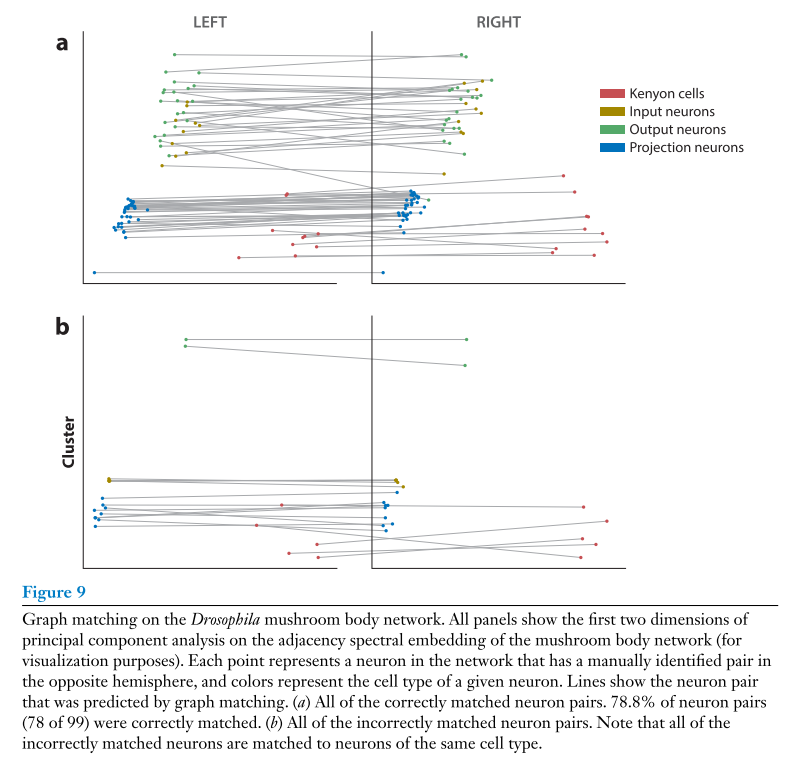
Application

In a recent paper, we applied these same tools for matching the nodes in the left and right Drosophila larva mushroom body connectome datasets, the same ones you get from graspologic.datasets.load_drosophila_left() etc.

Fig. 20 Figure from Chung et al. [4].

References

[1]

Jaewon Chung, Eric Bridgeford, Jesús Arroyo, Benjamin D Pedigo, Ali Saad-Eldin, Vivek Gopalakrishnan, Liang Xiang, Carey E Priebe, and Joshua T Vogelstein. Statistical connectomics. Annual Review of Statistics and Its Application, 8:463–492, 2021.

[2]

Joshua T Vogelstein, John M Conroy, Vince Lyzinski, Louis J Podrazik, Steven G Kratzer, Eric T Harley, Donniell E Fishkind, R Jacob Vogelstein, and Carey E Priebe. Fast approximate quadratic programming for graph matching. PLOS one, 10(4):e0121002, 2015.

[3] (1,2)

Donniell E Fishkind, Sancar Adali, Heather G Patsolic, Lingyao Meng, Digvijay Singh, Vince Lyzinski, and Carey E Priebe. Seeded graph matching. Pattern recognition, 87:203–215, 2019.