Analyzing Airport Data#
Author: Hope Ugwuoke
In this project I studied the data from all the flights in the US from September 1st to September 30th of 2021. I got this data from the Bureau of Transportation Statistics.
The nodes are aiports and the edges are flights. There are about 18,000 edges. The network is weighted because there are several flights (such as 100 or 200) flights between any two airports each month.
The network is directed because the flight come from an origin and have an end destination. Sometimes the weight becomes balenced because flights may come from an airport and then return to the airport.
When the weights are balenced the arrow is not visible. Yet there are some arrows in the image because some airports do not reciprocate. As in there are flights from the airport but no flights to the airport.
The first step was getting the data from the bureau of labor statistics and importing it into a networkx graph.
import pandas as pd
import numpy as np
import networkx as nx
import matplotlib.pyplot as plt
with open('Airport data.txt', 'r') as Flightdata:
    originlist = []
    destinationlist = []
    for i, row in enumerate(Flightdata):
        rowlist = row.split('|')
        originlist.append(rowlist[5])
        destinationlist.append(rowlist[16])

nodelist = np.unique(originlist)
flight_counts = pd.crosstab(originlist, destinationlist,dropna=False)
flight_counts = flight_counts.fillna(0)
for index in flight_counts.index:
    if index in flight_counts.columns:
        continue
    else:
        flight_counts[index]=np.zeros(435)
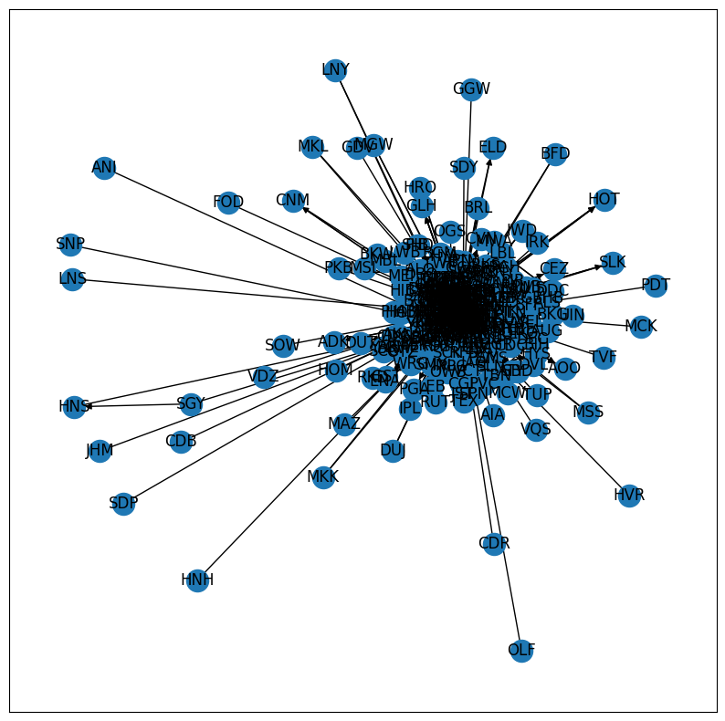
Initial plots of the Data#
G = nx.from_pandas_adjacency(flight_counts,create_using=nx.DiGraph)
fig, ax = plt.subplots(1,1,figsize=(10,10))
nx.draw_networkx(G)
from graspologic.plot import heatmap
adj = nx.to_numpy_array(G, nodelist=nodelist)

heatmap(adj, cbar=False)
<AxesSubplot: >
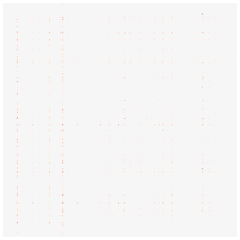
Observations:
The networkx graph is not very good
There are many smaller (less busy) airports that only fly to larger airports.
The large or busy airports are the lines that are visible on the graph.
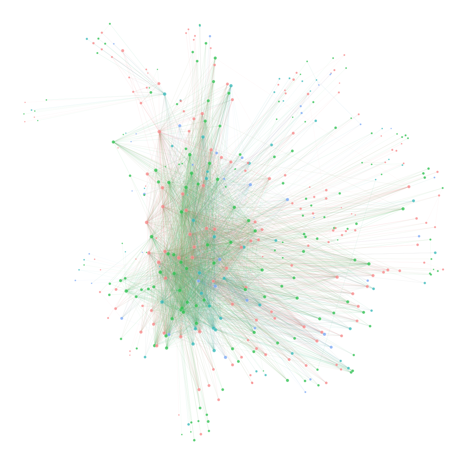
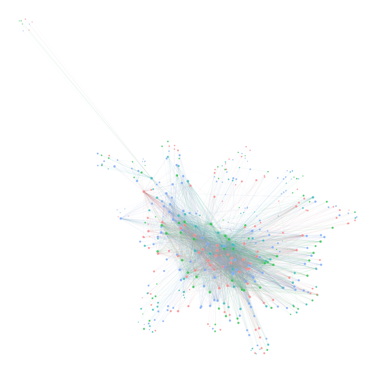
Community Detection#
Next I used leiden to detect communites and to create nicer looking plots.
Depending on resolution there could be anywhere from 3 to 45 communities. No matter the resolution the modularity was low. The modularity score for resolution of 1 was 0.18.
from graspologic.partition import leiden
from pathlib import Path
import pandas as pd
import networkx as nx
import numpy as np
from graspologic.layouts.colors import _get_colors
from sklearn.model_selection import ParameterGrid
from graspologic.embed import LaplacianSpectralEmbed
from graspologic.utils import pass_to_ranks
from umap import UMAP
from graspologic.plot import networkplot
from scipy.sparse import csr_array

main_random_state = np.random.default_rng(8888)
def symmetrze_nx(g):
    """Leiden requires a symmetric/undirected graph. This converts a directed graph to
    undirected just for this community detection step"""
    sym_g = nx.Graph()
    for source, target, weight in g.edges.data("weight"):
        if sym_g.has_edge(source, target):
            sym_g[source][target]["weight"] = (
                sym_g[source][target]["weight"] + weight * 0.5
            )
        else:
            sym_g.add_edge(source, target, weight=weight * 0.5)
    return sym_g
sym_G = symmetrze_nx(G)

out = leiden(sym_G, resolution = 1)
#making a series then a dataframe with leiden data
node_df = pd.Series(out)
node_df.index.name = "node_id"
node_df.name = "community"
node_df = node_df.to_frame()

#adding colors based on leiden communities
colors = _get_colors(True, None)["nominal"]
palette = dict(zip(node_df["community"].unique(), colors))

#graphing nodesize based on strength
adj = nx.to_scipy_sparse_array(G, nodelist=nodelist)
node_df["strength"] = adj.sum(axis=1) + adj.sum(axis=0)
node_df['rank_strength'] = node_df['strength'].rank(method='dense')

#Determining position
ptr_adj = pass_to_ranks(adj)
lse = LaplacianSpectralEmbed(n_components=32, concat=True)
lse_embedding = lse.fit_transform(adj)

n_components = 32
n_neighbors = 32
min_dist = 0.8
metric = "cosine"
umap = UMAP(
    n_components=2,
    n_neighbors=n_neighbors,
    min_dist=min_dist,
    metric=metric,
)
umap_embedding = umap.fit_transform(lse_embedding)
node_df["x"] = umap_embedding[:, 0]
node_df["y"] = umap_embedding[:, 1]

#Plotting using graspologic
ax = networkplot(
    adj,
    x="x",
    y="y",
    node_data=node_df,
    node_size="rank_strength",
    node_sizes=(10, 80),
    figsize=(20, 20),
    node_hue="community",
    edge_linewidth=0.3,
    palette=palette,
)
ax.axis("off")
(10.183902788162232, 26.191208791732787, -4.62498642206192, 9.912980568408965)
from graspologic.partition import leiden
from pathlib import Path
import pandas as pd
import networkx as nx
import numpy as np
from graspologic.layouts.colors import _get_colors
from sklearn.model_selection import ParameterGrid
from graspologic.embed import LaplacianSpectralEmbed
from graspologic.utils import pass_to_ranks
from umap import UMAP
from graspologic.plot import networkplot
from scipy.sparse import csr_array

main_random_state = np.random.default_rng(8888)
def symmetrze_nx(g):
    """Leiden requires a symmetric/undirected graph. This converts a directed graph to
    undirected just for this community detection step"""
    sym_g = nx.Graph()
    for source, target, weight in g.edges.data("weight"):
        if sym_g.has_edge(source, target):
            sym_g[source][target]["weight"] = (
                sym_g[source][target]["weight"] + weight * 0.5
            )
        else:
            sym_g.add_edge(source, target, weight=weight * 0.5)
    return sym_g
sym_G = symmetrze_nx(G)

out = leiden(sym_G, resolution = 3)
#making a series then a dataframe with leiden data
node_df = pd.Series(out)
node_df.index.name = "node_id"
node_df.name = "community"
node_df = node_df.to_frame()

#adding colors based on leiden communities
colors = _get_colors(True, None)["nominal"]
palette = dict(zip(node_df["community"].unique(), colors))

#graphing nodesize based on strength
adj = nx.to_scipy_sparse_array(G, nodelist=nodelist)
node_df["strength"] = adj.sum(axis=1) + adj.sum(axis=0)
node_df['rank_strength'] = node_df['strength'].rank(method='dense')

#Determining position
ptr_adj = pass_to_ranks(adj)
lse = LaplacianSpectralEmbed(n_components=32, concat=True)
lse_embedding = lse.fit_transform(adj)

n_components = 32
n_neighbors = 32
min_dist = 0.8
metric = "cosine"
umap = UMAP(
    n_components=2,
    n_neighbors=n_neighbors,
    min_dist=min_dist,
    metric=metric,
)
umap_embedding = umap.fit_transform(lse_embedding)
node_df["x"] = umap_embedding[:, 0]
node_df["y"] = umap_embedding[:, 1]

#Plotting using graspologic
ax = networkplot(
    adj,
    x="x",
    y="y",
    node_data=node_df,
    node_size="rank_strength",
    node_sizes=(10, 80),
    figsize=(20, 20),
    node_hue="community",
    edge_linewidth=0.3,
    palette=palette,
)
ax.axis("off")
(6.578326630592346, 22.542750430107116, -2.098478627204895, 12.844508957862853)
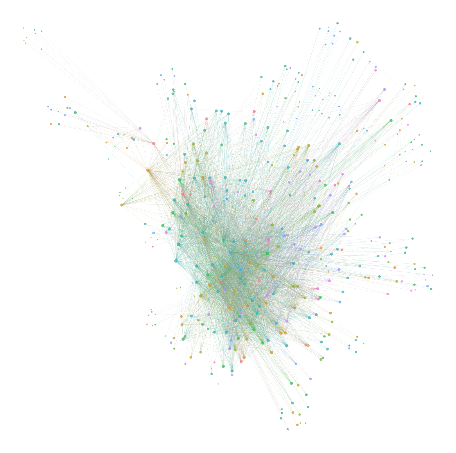
Even though the modularity was low, I wanted to explore if the communities had anything to do with geographic location. To do so, I sorted the data frame by community and strength to be able to investigate the most connected airports out of each community.
0 LNS, MLB, MDT, GSO, BNA PA, FL, PA NC TN 1 SGF, VPS, CMI, AEX, LFT Missouri, fl, Chicago, lousianna, lousianna 2 PSM, PBG, IAG, BMI, PGD new hamsphire, NY, NY, illinos, fl 3 PIR, RIW, SOW, DRO, VDZ
Sampling 5 airports from each community at resolutions 3 and looking at their geographic locations there were usually repeated states between each community.
HVN 2 105.0 47.0 20.941002 8.769190 FLL 2 152.0 55.0 19.784447 8.244032 MYR 2 5301.0 246.0 17.815920 6.894062 LBE conneticut, florida, SC, CA
IWD 4 757.0 134.0 20.121136 4.697268
TVC 4 855.0 139.0 18.464842 6.809649
PAH 4 1406.0 178.0 17.020662 -1.255356
SCE 4 1882.0 193.0 12.907616 2.366777
TBN
Michigan, michigan, kentucky, PA, Missouri
Looking at the data at a higher resolution there were still repeated cities in the data but the locations were generally not in a related geographic area. For example on community sampled had airports in Florida, Conneticut and California. This suggests that airports that are frequently flown to are not usually in the same geographic region. This makes sense because it would probably be cheaper to drive within short distance ranges. The exact way the communities are formed isn’t really clear.
node_df = node_df.sort_values(by=['community','strength'])
node_df
| community | strength | rank_strength | x | y | |
|---|---|---|---|---|---|
| node_id | |||||
| DAB | 0 | 1.0 | 1.0 | 14.213344 | 0.112244 |
| ATL | 0 | 3.0 | 3.0 | 10.702254 | 6.402745 |
| CSG | 0 | 7.0 | 7.0 | 13.378389 | 3.047507 |
| MGM | 0 | 45.0 | 21.0 | 17.104906 | 9.534023 |
| TLH | 0 | 46.0 | 22.0 | 17.120779 | -1.194793 |
| ... | ... | ... | ... | ... | ... |
| RUT | 43 | 41428.0 | 342.0 | 16.440046 | 1.811247 |
| PVC | 43 | 66484.0 | 356.0 | 15.186150 | 4.901760 |
| AUG | 43 | 161548.0 | 377.0 | 14.623292 | 2.648622 |
| BHB | 43 | 231327.0 | 384.0 | 11.721870 | 7.251369 |
| MEM | 44 | 7.0 | 7.0 | 7.388025 | 11.500373 |
435 rows × 5 columns
Some airports were very popular, and formed such strong communities that UMAP placed them very far away from the rest of the airports. These are probably cities near a major city so maybe a newark airport near New York City. It is difficult to tell exactly what these airports were as it changed everytime.
from graspologic.partition import leiden
from pathlib import Path
import pandas as pd
import networkx as nx
import numpy as np
from graspologic.layouts.colors import _get_colors
from sklearn.model_selection import ParameterGrid
from graspologic.embed import LaplacianSpectralEmbed
from graspologic.utils import pass_to_ranks
from umap import UMAP
from graspologic.plot import networkplot
from scipy.sparse import csr_array

main_random_state = np.random.default_rng(8888)
def symmetrze_nx(g):
    """Leiden requires a symmetric/undirected graph. This converts a directed graph to
    undirected just for this community detection step"""
    sym_g = nx.Graph()
    for source, target, weight in g.edges.data("weight"):
        if sym_g.has_edge(source, target):
            sym_g[source][target]["weight"] = (
                sym_g[source][target]["weight"] + weight * 0.5
            )
        else:
            sym_g.add_edge(source, target, weight=weight * 0.5)
    return sym_g
sym_G = symmetrze_nx(G)

out = leiden(sym_G, resolution = 1)
#making a series then a dataframe with leiden data
node_df = pd.Series(out)
node_df.index.name = "node_id"
node_df.name = "community"
node_df = node_df.to_frame()

#adding colors based on leiden communities
colors = _get_colors(True, None)["nominal"]
palette = dict(zip(node_df["community"].unique(), colors))

#graphing nodesize based on strength
adj = nx.to_scipy_sparse_array(G, nodelist=nodelist)
node_df["strength"] = adj.sum(axis=1) + adj.sum(axis=0)
node_df['rank_strength'] = node_df['strength'].rank(method='dense')

#Determining position
ptr_adj = pass_to_ranks(adj)
lse = LaplacianSpectralEmbed(n_components=32, concat=True)
lse_embedding = lse.fit_transform(adj)

n_components = 32
n_neighbors = 32
min_dist = 0.8
metric = "cosine"
umap = UMAP(
    n_components=2,
    n_neighbors=n_neighbors,
    min_dist=min_dist,
    metric=metric,
)
umap_embedding = umap.fit_transform(lse_embedding)
node_df["x"] = umap_embedding[:, 0]
node_df["y"] = umap_embedding[:, 1]

#Plotting using graspologic
ax = networkplot(
    adj,
    x="x",
    y="y",
    node_data=node_df,
    node_size="rank_strength",
    node_sizes=(10, 80),
    figsize=(20, 20),
    node_hue="community",
    edge_linewidth=0.3,
    palette=palette,
)
ax.axis("off")
(-2.6373936235904694,
 18.363856345415115,
 -5.282933330535888,
 15.767748928070068)
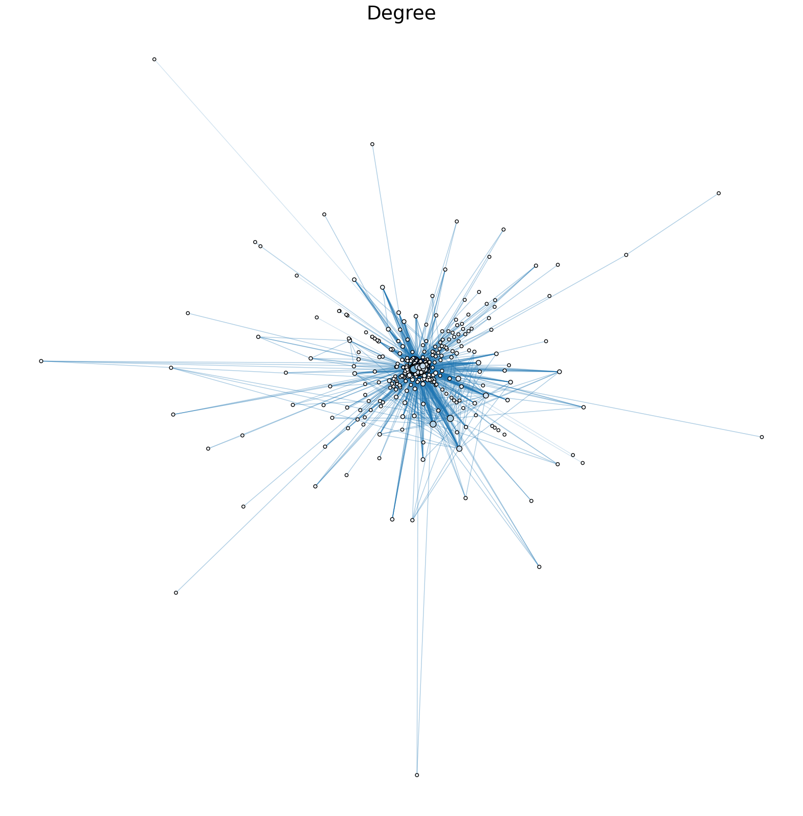
Centrality Measures#
Next I tried the different centrality measures on the data.
Looking at the centrality based on degree, it is clear that there are a few incredibly densly connnected airports that are in the center of the diagram.
import pandas as pd
import matplotlib.pyplot as plt
from graspologic.plot import networkplot
import seaborn as sns
from matplotlib import colors
import networkx as nx
A = nx.to_scipy_sparse_array(G, nodelist=nodelist)
node_data = pd.DataFrame(index=G.nodes())
node_data["degree"] = node_data.index.map(dict(nx.degree(G)))

pos = nx.kamada_kawai_layout(G)
node_data["x"] = [pos[node][0] for node in node_data.index]
node_data["y"] = [pos[node][1] for node in node_data.index]

sns.set_context("talk", font_scale=1.5)
fig, axs = plt.subplots(1, 1, figsize=(20, 20))


def plot_node_scaled_network(A, node_data, key, ax):
    # REF: https://github.com/mwaskom/seaborn/blob/9425588d3498755abd93960df4ab05ec1a8de3ef/seaborn/_core.py#L215

    levels = list(np.sort(node_data[key].unique()))
    cmap = sns.color_palette("Blues", as_cmap=True)
    vmin = np.min(levels)
    norm = colors.Normalize(vmin=0.3 * vmin)
    palette = dict(zip(levels, cmap(norm(levels))))

    networkplot(
        A,
        node_data=node_data,
        x="x",
        y="y",
        ax=ax,
        edge_linewidth=1.0,
        node_size=key,
        node_hue=key,
        palette=palette,
        node_sizes=(20, 200),
        node_kws=dict(linewidth=1, edgecolor="black"),
        node_alpha=1.0,
        edge_kws=dict(color=sns.color_palette()[0]),
    )

    ax.axis("off")
    ax.set_title(key.capitalize())

ax = axs
plot_node_scaled_network(A, node_data, "degree", ax)

fig.set_facecolor("w")
I then compared all the centrality measures in the same graph. This code was based on code by Ben Pedigo.
import pandas as pd
import matplotlib.pyplot as plt
from graspologic.plot import networkplot
import seaborn as sns
from matplotlib import colors
import networkx as nx
A = nx.to_scipy_sparse_array(G, nodelist=nodelist)
node_data = pd.DataFrame(index=G.nodes())
node_data["degree"] = node_data.index.map(dict(nx.degree(G)))
node_data["eigenvector"] = node_data.index.map(nx.eigenvector_centrality(G))
node_data["pagerank"] = node_data.index.map(nx.pagerank(G))
node_data["betweenness"] = node_data.index.map(nx.betweenness_centrality(G))

pos = nx.kamada_kawai_layout(G)
node_data["x"] = [pos[node][0] for node in node_data.index]
node_data["y"] = [pos[node][1] for node in node_data.index]

sns.set_context("talk", font_scale=1.5)
fig, axs = plt.subplots(1, 4, figsize=(20, 5))


def plot_node_scaled_network(A, node_data, key, ax):
    # REF: https://github.com/mwaskom/seaborn/blob/9425588d3498755abd93960df4ab05ec1a8de3ef/seaborn/_core.py#L215

    levels = list(np.sort(node_data[key].unique()))
    cmap = sns.color_palette("Blues", as_cmap=True)
    vmin = np.min(levels)
    norm = colors.Normalize(vmin=0.3 * vmin)
    palette = dict(zip(levels, cmap(norm(levels))))

    networkplot(
        A,
        node_data=node_data,
        x="x",
        y="y",
        ax=ax,
        edge_linewidth=1.0,
        node_size=key,
        node_hue=key,
        palette=palette,
        node_sizes=(20, 200),
        node_kws=dict(linewidth=1, edgecolor="black"),
        node_alpha=1.0,
        edge_kws=dict(color=sns.color_palette()[0]),
    )

    ax.axis("off")
    ax.set_title(key.capitalize())


ax = axs[0]
plot_node_scaled_network(A, node_data, "degree", ax)

ax = axs[1]
plot_node_scaled_network(A, node_data, "eigenvector", ax)

ax = axs[2]
plot_node_scaled_network(A, node_data, "pagerank", ax)

ax = axs[3]
plot_node_scaled_network(A, node_data, "betweenness", ax)

fig.set_facecolor("w")
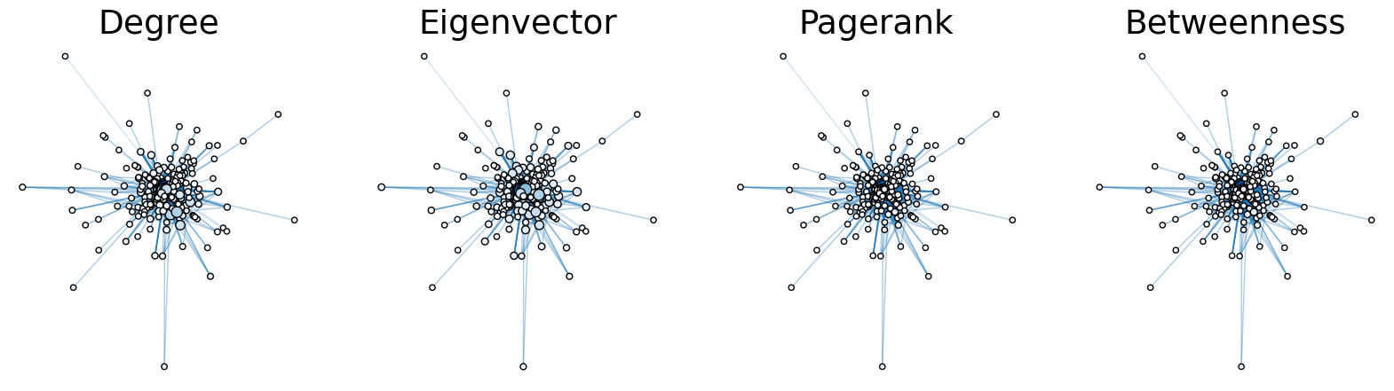
I used .sort_values() to rank the airports based on the different centrality measures. Then I manually added the top 10 airports to sets in order to conduct set operations.
node_data = node_data.sort_values(by=['degree'])
degree = {'LAX','IAH','MSP','PHX','CLT', 'LAS', 'ATL', 'DEN', 'ORD', 'DFW'}
eigenvector = {'MDW', 'MSP','BNA', 'PHX', 'CLT', 'ATL', 'LAS','DFW','DEN','ORD'}
betweenness = {'SLC','MSP', 'PHX','LAX','LAS','SEA','CLT','ORD','DFW','ATL','DEN'}
pagerank = {'SLC','LAS','SEA','MSP','CLT','ATL','ANC','DEN','ORD','DFW'}

ConnectedAiports = degree & eigenvector
connectedaiports = betweenness & pagerank
connectedAirports = connectedaiports & ConnectedAiports

print(connectedAirports)
{'LAS', 'DFW', 'ORD', 'ATL', 'CLT', 'MSP', 'DEN'}
There were 6 airports that appeared in every centrality measure:
Las Vegas, Atlanta, Dallas/Fort worth, Chicago O’hare, Charlotte, Minneapolis and Denver.
The consistency between the centrality measures verifies that these airports are very highly connected. Looking at the airports it makes sense based on populaton of the cities in which these airports are located.
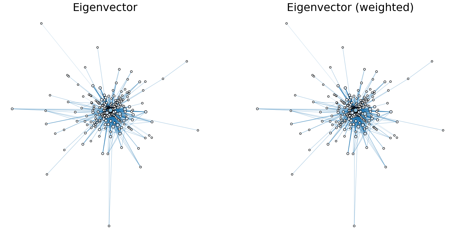
These centrality measures did not account for the weight of each connection in the graph. So I compared the eigenvector plots when it was weighted and unweighted.
import pandas as pd
import matplotlib.pyplot as plt
from graspologic.plot import networkplot
import seaborn as sns
from matplotlib import colors
import networkx as nx
A = nx.to_scipy_sparse_array(G, nodelist=nodelist)
node_data = pd.DataFrame(index=G.nodes())
node_data["eigenvector"] = node_data.index.map(nx.eigenvector_centrality(G))
node_data["eigenvector (weighted)"] = node_data.index.map(nx.eigenvector_centrality(G))

pos = nx.kamada_kawai_layout(G)
node_data["x"] = [pos[node][0] for node in node_data.index]
node_data["y"] = [pos[node][1] for node in node_data.index]

sns.set_context("talk", font_scale=1.5)
fig, axs = plt.subplots(1, 2, figsize=(20, 10))


def plot_node_scaled_network(A, node_data, key, ax):
    # REF: https://github.com/mwaskom/seaborn/blob/9425588d3498755abd93960df4ab05ec1a8de3ef/seaborn/_core.py#L215

    levels = list(np.sort(node_data[key].unique()))
    cmap = sns.color_palette("Blues", as_cmap=True)
    vmin = np.min(levels)
    norm = colors.Normalize(vmin=0.3 * vmin)
    palette = dict(zip(levels, cmap(norm(levels))))

    networkplot(
        A,
        node_data=node_data,
        x="x",
        y="y",
        ax=ax,
        edge_linewidth=1.0,
        node_size=key,
        node_hue=key,
        palette=palette,
        node_sizes=(20, 200),
        node_kws=dict(linewidth=1, edgecolor="black"),
        node_alpha=1.0,
        edge_kws=dict(color=sns.color_palette()[0]),
    )

    ax.axis("off")
    ax.set_title(key.capitalize())


ax = axs[0]
plot_node_scaled_network(A, node_data, "eigenvector", ax)

ax = axs[1]
plot_node_scaled_network(A, node_data, "eigenvector (weighted)", ax)

fig.set_facecolor("w")
node_data = node_data.sort_values(by=['eigenvector (weighted)'])
print(node_data.to_string())
eigenvector eigenvector (weighted) x y
JMS 1.277276e-21 1.277276e-21 -0.231443 0.227580
DUJ 1.277276e-21 1.277276e-21 -0.000657 0.009819
PDT 1.277276e-21 1.277276e-21 0.022719 -0.023362
CYS 1.277276e-21 1.277276e-21 -0.506314 0.759154
PKB 1.277276e-21 1.277276e-21 0.067229 -0.072572
HRO 1.277276e-21 1.277276e-21 -0.011257 0.017871
JHM 1.277276e-21 1.277276e-21 0.011682 -0.005062
PVC 1.277276e-21 1.277276e-21 0.157823 -0.152436
IWD 1.277276e-21 1.277276e-21 -0.017577 0.018111
DVL 1.277276e-21 1.277276e-21 -0.148734 0.140681
RKD 1.277276e-21 1.277276e-21 0.076887 -0.084109
CDR 1.277276e-21 1.277276e-21 0.030904 0.001687
CDB 1.277276e-21 1.277276e-21 -0.039658 0.003241
RUT 1.277276e-21 1.277276e-21 0.090060 -0.097902
HVR 1.277276e-21 1.277276e-21 -0.080893 0.072872
SDP 1.277276e-21 1.277276e-21 -0.025902 0.002085
SDY 1.277276e-21 1.277276e-21 -0.097682 0.088094
SGY 1.277276e-21 1.277276e-21 -0.130907 0.073230
BRL 1.277276e-21 1.277276e-21 -0.016720 0.019398
IRK 1.277276e-21 1.277276e-21 -0.085671 0.077441
SNP 1.277276e-21 1.277276e-21 -0.025902 0.002085
EAU 1.277276e-21 1.277276e-21 -0.009475 0.004340
OGS 1.277276e-21 1.277276e-21 0.169605 -0.163213
LBF 1.277276e-21 1.277276e-21 -0.311727 0.309987
LEB 1.277276e-21 1.277276e-21 -0.049926 0.046108
LNS 1.277276e-21 1.277276e-21 -0.000658 0.009819
LNY 1.277276e-21 1.277276e-21 0.012333 -0.004246
HNH 1.277276e-21 1.277276e-21 -0.129033 0.070673
MAZ 1.277276e-21 1.277276e-21 0.030316 -0.030414
GGW 1.277276e-21 1.277276e-21 -0.080922 0.072834
MBL 1.277276e-21 1.277276e-21 -0.149763 0.140450
OLF 1.277276e-21 1.277276e-21 -0.075781 0.068516
GDV 1.277276e-21 1.277276e-21 -0.085995 0.077087
MCK 1.277276e-21 1.277276e-21 0.045448 -0.018541
FOD 1.277276e-21 1.277276e-21 0.000930 0.020860
MGW 1.277276e-21 1.277276e-21 -0.000655 0.009820
MKK 1.277276e-21 1.277276e-21 0.013916 -0.008072
MKL 1.277276e-21 1.277276e-21 -0.003068 0.010465
MSL 1.277276e-21 1.277276e-21 0.114318 -0.115705
MSS 1.277276e-21 1.277276e-21 -0.003993 0.012810
MWA 1.277276e-21 1.277276e-21 0.057351 -0.062909
HOM 1.277276e-21 1.277276e-21 -0.192789 0.124796
SOW 1.277276e-21 1.277276e-21 0.025322 -0.028470
PUB 1.277276e-21 1.277276e-21 0.301743 -0.213473
ANI 1.277276e-21 1.277276e-21 -0.025902 0.002085
TVF 1.277276e-21 1.277276e-21 0.036940 -0.041612
VDZ 1.277276e-21 1.277276e-21 -0.111867 0.039316
TUP 1.277276e-21 1.277276e-21 0.072180 -0.079022
AIA 1.277276e-21 1.277276e-21 0.082854 -0.079489
AUG 1.277276e-21 1.277276e-21 0.145959 -0.142131
BFD 1.277276e-21 1.277276e-21 -0.000658 0.009819
TBN 1.277276e-21 1.277276e-21 0.018527 0.066588
IPL 1.277276e-21 1.277276e-21 0.008435 -0.008355
VQS 1.277276e-21 1.277276e-21 0.038391 -0.039925
VCT 1.277276e-21 1.277276e-21 0.320489 -0.232897
BHB 1.277276e-21 1.277276e-21 0.150763 -0.146206
UIN 1.277276e-21 1.277276e-21 0.033835 -0.033533
HNS 1.532731e-20 1.532731e-20 -0.129363 0.070717
BFF 1.532731e-20 1.532731e-20 -0.301473 0.299727
DDC 2.615860e-18 2.615860e-18 -0.133686 0.129605
LBL 2.615860e-18 2.615860e-18 -0.135786 0.131579
SPN 1.383288e-05 1.383288e-05 0.583097 0.429985
PIB 3.533875e-05 3.533875e-05 -0.011019 -0.041064
DEC 4.156471e-05 4.156471e-05 0.014854 0.040547
JST 9.785644e-05 9.785644e-05 0.012103 0.026688
ENA 5.369901e-04 5.369901e-04 -0.017109 -0.000711
DLG 5.369901e-04 5.369901e-04 -0.441606 0.135264
AKN 5.369901e-04 5.369901e-04 0.666337 -0.169218
OME 5.369901e-04 5.369901e-04 -0.402457 -0.197675
ADQ 5.369901e-04 5.369901e-04 -0.464561 -0.551817
SCC 5.369901e-04 5.369901e-04 -0.334447 -0.340066
BET 5.369901e-04 5.369901e-04 -0.085532 0.550594
BRW 5.369901e-04 5.369901e-04 -0.178289 0.377985
DUT 5.369901e-04 5.369901e-04 -0.016935 -0.000672
ADK 5.369901e-04 5.369901e-04 -0.099322 -0.038985
OTZ 5.456055e-04 5.456055e-04 -0.336315 -0.165208
OWB 6.032396e-04 6.032396e-04 0.049612 -0.052472
PPG 8.619476e-04 8.619476e-04 -0.135293 -0.262823
GUM 8.621695e-04 8.621695e-04 0.404509 0.278452
ELD 1.070830e-03 1.070830e-03 0.000989 0.013960
CNM 1.296874e-03 1.296874e-03 -0.005029 -0.008506
HYA 1.605130e-03 1.605130e-03 -0.018217 0.024825
SLK 1.605130e-03 1.605130e-03 0.028589 -0.027377
IAG 1.612371e-03 1.612371e-03 -0.474046 0.001054
BIH 1.866664e-03 1.866664e-03 0.018571 0.107008
SBD 1.866664e-03 1.866664e-03 -0.027831 -0.151003
PQI 1.895676e-03 1.895676e-03 -0.102766 -0.138516
PIH 1.905395e-03 1.905395e-03 -0.037466 -0.038855
CDC 1.905395e-03 1.905395e-03 0.086657 0.054057
EKO 1.905395e-03 1.905395e-03 -0.038564 -0.032750
WYS 1.905395e-03 1.905395e-03 0.128097 -0.042465
BTM 1.905395e-03 1.905395e-03 0.012100 0.056567
TWF 1.905395e-03 1.905395e-03 0.041632 0.037988
ART 1.955433e-03 1.955433e-03 0.058294 0.046751
YKM 1.985193e-03 1.985193e-03 0.080622 0.083222
ALW 1.985193e-03 1.985193e-03 0.272519 0.254120
EAT 1.985193e-03 1.985193e-03 0.089614 0.096492
GST 2.030258e-03 2.030258e-03 -0.041454 -0.027477
BGM 2.118176e-03 2.118176e-03 0.101253 0.043905
MEI 2.202442e-03 2.202442e-03 0.018022 0.000818
INL 2.230904e-03 2.230904e-03 -0.099264 -0.065581
ABR 2.230904e-03 2.230904e-03 0.061294 0.090893
HIB 2.230904e-03 2.230904e-03 -0.044372 -0.026206
BJI 2.230904e-03 2.230904e-03 0.050347 0.070108
TEX 2.260773e-03 2.260773e-03 -0.002545 -0.015159
PGA 2.260773e-03 2.260773e-03 -0.010270 -0.020632
CEZ 2.260773e-03 2.260773e-03 -0.000527 -0.020325
BRD 2.266699e-03 2.266699e-03 0.045680 0.063318
LYH 2.269786e-03 2.269786e-03 -0.032205 -0.043934
FLO 2.269786e-03 2.269786e-03 0.021014 0.005734
PGV 2.269786e-03 2.269786e-03 -0.031830 -0.047031
PHF 2.269786e-03 2.269786e-03 -0.100104 -0.120695
BKW 2.269786e-03 2.269786e-03 0.019507 0.001776
HGR 2.398962e-03 2.398962e-03 -0.162960 -0.121923
VLD 2.508599e-03 2.508599e-03 0.057168 0.050358
BQK 2.508599e-03 2.508599e-03 0.256391 0.177489
ABY 2.508599e-03 2.508599e-03 0.036753 0.029061
GTR 2.508599e-03 2.508599e-03 -0.088662 -0.102855
DHN 2.508599e-03 2.508599e-03 0.106114 0.097084
SMX 2.521970e-03 2.521970e-03 0.249798 0.066288
SJT 2.539220e-03 2.539220e-03 0.151509 0.167214
GRK 2.539220e-03 2.539220e-03 -0.051026 -0.048032
ACT 2.539220e-03 2.539220e-03 0.044281 0.047687
GGG 2.539220e-03 2.539220e-03 -0.041242 -0.020230
BPT 2.539220e-03 2.539220e-03 0.087510 0.108934
ABI 2.539220e-03 2.539220e-03 0.072470 0.076908
GCK 2.539220e-03 2.539220e-03 0.099874 0.131701
FSM 2.539220e-03 2.539220e-03 0.135208 0.158151
SPS 2.539220e-03 2.539220e-03 0.030699 0.040861
SWO 2.539220e-03 2.539220e-03 0.062544 0.070630
CLL 2.539220e-03 2.539220e-03 0.150551 0.150706
LAW 2.539220e-03 2.539220e-03 -0.047378 -0.037775
CVN 2.539220e-03 2.539220e-03 -0.008112 0.039649
DRT 2.539220e-03 2.539220e-03 0.120432 0.187323
TYR 2.539220e-03 2.539220e-03 0.048719 0.054431
COD 2.575752e-03 2.575752e-03 0.140400 0.273665
GCC 2.575752e-03 2.575752e-03 0.017816 0.009618
SHR 2.575752e-03 2.575752e-03 0.020972 0.011627
RKS 2.575752e-03 2.575752e-03 0.018203 0.009456
LAR 2.575752e-03 2.575752e-03 0.018135 0.009542
RIW 2.575752e-03 2.575752e-03 0.018330 0.009352
PIR 2.575752e-03 2.575752e-03 0.018549 0.009209
BKG 2.575752e-03 2.575752e-03 0.178241 0.007288
DIK 2.575752e-03 2.575752e-03 0.092816 0.167914
ALS 2.575752e-03 2.575752e-03 0.023083 0.011179
VEL 2.575752e-03 2.575752e-03 0.018769 0.008995
ATY 2.590406e-03 2.590406e-03 0.020300 0.021469
DBQ 2.590406e-03 2.590406e-03 -0.044576 -0.044878
EAR 2.590406e-03 2.590406e-03 0.013866 0.012962
MKG 2.590406e-03 2.590406e-03 0.013740 0.012380
ALO 2.590406e-03 2.590406e-03 0.081138 0.066143
CGI 2.590406e-03 2.590406e-03 0.013881 0.013556
MCW 2.590406e-03 2.590406e-03 0.017711 0.017191
CMX 2.590406e-03 2.590406e-03 0.017339 0.014329
YAK 2.609111e-03 2.609111e-03 -0.071848 0.027341
CDV 2.609111e-03 2.609111e-03 -0.065548 0.028619
SIT 2.610477e-03 2.610477e-03 -0.305712 0.077095
PAH 2.631971e-03 2.631971e-03 0.016970 0.015054
PSG 2.653044e-03 2.653044e-03 -0.121058 0.004768
WRG 2.653044e-03 2.653044e-03 -0.112055 0.021869
SHD 2.660537e-03 2.660537e-03 0.007507 0.016909
HYS 2.673988e-03 2.673988e-03 0.016243 0.020068
KTN 2.694267e-03 2.694267e-03 -0.204439 0.024148
JNU 2.808731e-03 2.808731e-03 -0.129135 0.067742
PUW 3.064268e-03 3.064268e-03 -0.072023 -0.221181
PBG 3.096278e-03 3.096278e-03 0.272258 -0.235963
ELM 3.263790e-03 3.263790e-03 0.030447 0.177557
USA 3.563035e-03 3.563035e-03 0.236679 -0.488269
HOT 3.610050e-03 3.610050e-03 -0.001392 0.011305
AOO 3.706454e-03 3.706454e-03 -0.009199 0.006587
PSE 3.775109e-03 3.775109e-03 0.000652 -1.000000
TOL 4.202777e-03 4.202777e-03 0.111448 0.040384
SBY 4.225219e-03 4.225219e-03 -0.014962 -0.015368
CIU 4.349080e-03 4.349080e-03 -0.036720 0.010928
RHI 4.349080e-03 4.349080e-03 -0.017779 -0.003811
ESC 4.349080e-03 4.349080e-03 -0.038267 0.003479
LWB 4.370799e-03 4.370799e-03 0.003364 0.017774
EWN 4.395763e-03 4.395763e-03 0.034689 0.014128
PLN 4.418862e-03 4.418862e-03 -0.019538 0.002057
IMT 4.418862e-03 4.418862e-03 -0.018181 -0.007040
APN 4.418862e-03 4.418862e-03 -0.019111 0.005865
OTH 4.442416e-03 4.442416e-03 0.012957 -0.182342
CNY 4.481147e-03 4.481147e-03 0.019369 0.008665
CPR 4.481147e-03 4.481147e-03 0.049407 0.090721
LWS 4.481147e-03 4.481147e-03 -0.179697 -0.090784
RFD 4.521837e-03 4.521837e-03 -0.008230 -0.373519
MBS 4.708582e-03 4.708582e-03 -0.026154 -0.019705
MQT 4.708582e-03 4.708582e-03 -0.092470 -0.080696
AZO 4.708582e-03 4.708582e-03 0.030773 0.032229
BRO 4.741095e-03 4.741095e-03 0.167782 0.340885
TXK 4.741095e-03 4.741095e-03 0.046050 0.019890
LCH 4.741095e-03 4.741095e-03 -0.038041 -0.037732
GFK 4.752874e-03 4.752874e-03 -0.252439 -0.011048
PRC 4.754323e-03 4.754323e-03 0.016939 0.004346
GUC 4.777627e-03 4.777627e-03 -0.035292 0.066557
HOB 4.777627e-03 4.777627e-03 -0.072974 -0.034608
OAJ 4.778385e-03 4.778385e-03 -0.070757 -0.080633
SCK 4.782743e-03 4.782743e-03 0.221466 -0.326148
GLH 4.796539e-03 4.796539e-03 -0.006682 0.024826
ROW 4.799993e-03 4.799993e-03 0.144225 0.094430
YUM 4.799993e-03 4.799993e-03 0.076045 0.119072
DLH 4.821310e-03 4.821310e-03 0.069456 0.087163
RST 4.821310e-03 4.821310e-03 -0.028393 -0.018881
LSE 4.821310e-03 4.821310e-03 -0.030922 -0.021719
ERI 4.860192e-03 4.860192e-03 0.139561 0.123084
MLU 5.047819e-03 5.047819e-03 -0.108782 -0.103082
AEX 5.047819e-03 5.047819e-03 0.078355 0.105670
EGE 5.114972e-03 5.114972e-03 0.093936 0.083556
PSM 5.123037e-03 5.123037e-03 0.041917 -0.103949
MHK 5.129626e-03 5.129626e-03 -0.132499 -0.147540
CMI 5.129626e-03 5.129626e-03 0.100233 0.091046
COU 5.129626e-03 5.129626e-03 0.077514 0.360654
SUX 5.166158e-03 5.166158e-03 0.024863 0.014854
JLN 5.166158e-03 5.166158e-03 0.021900 0.012831
SLN 5.209064e-03 5.209064e-03 0.019220 0.010777
LBE 5.373991e-03 5.373991e-03 -0.469918 -0.113866
GRI 5.448687e-03 5.448687e-03 -0.238954 -0.090229
ORH 5.631981e-03 5.631981e-03 -0.166913 -0.044568
ITH 5.969286e-03 5.969286e-03 -0.039926 -0.052215
SPI 5.983879e-03 5.983879e-03 0.069302 0.041806
CKB 6.098630e-03 6.098630e-03 0.011558 0.017493
HTS 6.243197e-03 6.243197e-03 -0.018977 -0.055391
HLN 6.466340e-03 6.466340e-03 -0.134099 -0.096696
AVP 6.755868e-03 6.755868e-03 0.035846 0.052799
LAN 6.834559e-03 6.834559e-03 -0.016663 -0.009520
CWA 6.939486e-03 6.939486e-03 -0.017864 -0.009081
LRD 7.263065e-03 7.263065e-03 -0.065159 -0.083997
ITO 7.279387e-03 7.279387e-03 -0.021415 -0.007135
CSG 7.317605e-03 7.317605e-03 -0.013040 -0.014530
FAY 7.317605e-03 7.317605e-03 -0.021118 -0.031535
XWA 7.328626e-03 7.328626e-03 0.001684 -0.033778
SAF 7.375745e-03 7.375745e-03 -0.176803 -0.192770
FLG 7.375745e-03 7.375745e-03 -0.069004 -0.093504
BQN 7.621450e-03 7.621450e-03 -0.724804 0.017426
MOT 7.716123e-03 7.716123e-03 0.094483 -0.319197
TRI 8.463219e-03 8.463219e-03 0.067193 0.026779
SCE 8.559692e-03 8.559692e-03 -0.032874 -0.042119
CHO 8.592275e-03 8.592275e-03 0.033311 0.039276
LNK 8.604755e-03 8.604755e-03 -0.024166 -0.022214
MLB 8.685919e-03 8.685919e-03 0.077931 -0.157598
EVV 9.028537e-03 9.028537e-03 0.009448 0.015621
FAI 9.192029e-03 9.192029e-03 -0.003169 -0.006680
GNV 9.208952e-03 9.208952e-03 0.055188 0.242508
BFL 9.242409e-03 9.242409e-03 0.053260 0.052867
DAB 9.273038e-03 9.273038e-03 -0.017511 0.070362
SGU 9.281140e-03 9.281140e-03 0.017943 0.009590
MGM 9.443582e-03 9.443582e-03 0.014717 -0.026178
AGS 9.443582e-03 9.443582e-03 0.047970 0.030539
MOB 9.519480e-03 9.519480e-03 -0.195563 -0.290394
BTR 9.519480e-03 9.519480e-03 0.230381 0.251932
LFT 9.519480e-03 9.519480e-03 -0.114016 -0.125970
RDD 9.755464e-03 9.755464e-03 0.095175 -0.144643
STX 9.773266e-03 9.773266e-03 0.048969 -0.006639
DRO 9.897715e-03 9.897715e-03 -0.080707 -0.008233
MFE 1.004488e-02 1.004488e-02 0.023928 -0.016757
ACV 1.008483e-02 1.008483e-02 0.169917 -0.005869
BLV 1.009231e-02 1.009231e-02 -0.001438 0.127741
BIS 1.085858e-02 1.085858e-02 0.322295 -0.096047
HDN 1.092071e-02 1.092071e-02 -0.002537 0.003399
LCK 1.097158e-02 1.097158e-02 -0.003312 -0.050618
GTF 1.157872e-02 1.157872e-02 -0.031902 0.094828
CRW 1.166475e-02 1.166475e-02 0.037685 0.129826
PAE 1.201063e-02 1.201063e-02 -0.047120 -0.371438
GPT 1.235362e-02 1.235362e-02 -0.027906 0.020299
SWF 1.251334e-02 1.251334e-02 0.086536 -0.045126
SUN 1.310198e-02 1.310198e-02 0.121815 -0.008539
GJT 1.328064e-02 1.328064e-02 -0.015506 -0.012780
BLI 1.410973e-02 1.410973e-02 -0.001663 0.006882
BMI 1.458546e-02 1.458546e-02 -0.032314 0.035991
MVY 1.461091e-02 1.461091e-02 0.063698 -0.025465
GRB 1.477357e-02 1.477357e-02 -0.009746 0.020276
TTN 1.484518e-02 1.484518e-02 0.175534 -0.078460
SBP 1.503164e-02 1.503164e-02 0.021109 -0.028843
TLH 1.532414e-02 1.532414e-02 0.004338 -0.029628
MRY 1.592814e-02 1.592814e-02 0.031920 -0.016698
CRP 1.609723e-02 1.609723e-02 0.003830 -0.000832
CAK 1.612501e-02 1.612501e-02 -0.034636 0.136546
MTJ 1.622917e-02 1.622917e-02 0.004419 0.014497
ACY 1.642636e-02 1.642636e-02 0.112178 -0.086117
ROA 1.654105e-02 1.654105e-02 0.012833 -0.087907
MLI 1.657922e-02 1.657922e-02 -0.071339 -0.162520
CHA 1.718912e-02 1.718912e-02 -0.026833 0.053496
FNT 1.722427e-02 1.722427e-02 -0.119568 -0.013047
RDM 1.737658e-02 1.737658e-02 -0.003611 0.011628
BGR 1.765220e-02 1.765220e-02 0.077323 0.036628
STS 1.768909e-02 1.768909e-02 0.008704 -0.010265
FAR 1.788488e-02 1.788488e-02 -0.120420 0.217645
BIL 1.836181e-02 1.836181e-02 -0.073389 0.066569
ASE 1.841334e-02 1.841334e-02 -0.003828 -0.014523
SHV 1.850670e-02 1.850670e-02 0.153908 0.035428
ACK 1.868058e-02 1.868058e-02 -0.019461 0.020064
PVU 1.883516e-02 1.883516e-02 -0.004608 -0.117244
ABE 1.883889e-02 1.883889e-02 0.181352 -0.034297
PSC 1.885454e-02 1.885454e-02 0.012234 -0.224511
CAE 2.030343e-02 2.030343e-02 -0.015960 -0.020286
PIA 2.085601e-02 2.085601e-02 -0.026824 -0.119076
DAY 2.153386e-02 2.153386e-02 -0.052708 -0.030712
HHH 2.168698e-02 2.168698e-02 0.011170 -0.027610
IDA 2.187537e-02 2.187537e-02 -0.024282 0.114588
MFR 2.190612e-02 2.190612e-02 0.013631 -0.007764
LEX 2.203167e-02 2.203167e-02 -0.022739 -0.084781
HVN 2.208435e-02 2.208435e-02 -0.065911 0.198899
LIH 2.212996e-02 2.212996e-02 -0.005905 0.006482
SGF 2.249374e-02 2.249374e-02 0.275717 -0.008703
GSO 2.251318e-02 2.251318e-02 -0.039492 -0.070756
FWA 2.303105e-02 2.303105e-02 -0.022153 -0.011438
ATW 2.303188e-02 2.303188e-02 0.022250 -0.005594
AZA 2.415169e-02 2.415169e-02 0.133729 -0.067096
ILM 2.452983e-02 2.452983e-02 -0.054726 0.095847
RAP 2.545544e-02 2.545544e-02 0.014977 -0.018593
HPN 2.558634e-02 2.558634e-02 -0.047141 0.046250
SBN 2.711317e-02 2.711317e-02 0.009732 0.001424
BTV 2.822895e-02 2.822895e-02 -0.012836 0.016829
MSO 2.828754e-02 2.828754e-02 -0.008006 -0.028224
STT 2.861349e-02 2.861349e-02 0.036733 -0.011787
KOA 2.899000e-02 2.899000e-02 0.005567 0.009391
PGD 2.909175e-02 2.909175e-02 0.082416 -0.197813
CID 2.909468e-02 2.909468e-02 -0.006615 0.008838
FSD 2.911595e-02 2.911595e-02 0.008041 0.009999
FCA 2.930821e-02 2.930821e-02 0.014190 -0.010473
JAC 3.032708e-02 3.032708e-02 0.003549 -0.014366
HSV 3.124000e-02 3.124000e-02 0.008449 -0.014951
TVC 3.172025e-02 3.172025e-02 0.012882 -0.001198
MDT 3.261988e-02 3.261988e-02 0.000458 0.017134
FAT 3.277092e-02 3.277092e-02 0.004274 0.007714
SBA 3.306616e-02 3.306616e-02 0.008150 -0.003317
ANC 3.346730e-02 3.346730e-02 -0.017293 0.001639
PIE 3.380542e-02 3.380542e-02 0.031708 -0.137508
EUG 3.464327e-02 3.464327e-02 0.003834 0.006424
EYW 3.475285e-02 3.475285e-02 0.012316 -0.038661
JAN 3.617716e-02 3.617716e-02 -0.005735 0.004722
OGG 3.678101e-02 3.678101e-02 0.016720 -0.003240
SFB 3.759879e-02 3.759879e-02 0.065059 -0.123355
XNA 3.794049e-02 3.794049e-02 -0.013806 -0.017302
LBB 3.977900e-02 3.977900e-02 0.004725 0.002729
MHT 4.038688e-02 4.038688e-02 -0.001015 -0.001821
PSP 4.090763e-02 4.090763e-02 0.007841 0.001597
ICT 4.165485e-02 4.165485e-02 -0.002075 -0.006724
HRL 4.266620e-02 4.266620e-02 0.002698 -0.002981
ISP 4.292413e-02 4.292413e-02 0.010726 -0.000022
AMA 4.292440e-02 4.292440e-02 0.006907 0.000502
MSN 4.432352e-02 4.432352e-02 -0.004511 -0.006794
AVL 4.453640e-02 4.453640e-02 0.119398 0.013593
LIT 4.624831e-02 4.624831e-02 -0.001064 -0.004048
PBI 4.675654e-02 4.675654e-02 0.007300 0.013530
MAF 4.956223e-02 4.956223e-02 0.000312 0.005210
ECP 5.269266e-02 5.269266e-02 0.000876 0.001880
TYS 5.280044e-02 5.280044e-02 0.080523 -0.025632
PNS 5.282685e-02 5.282685e-02 0.005240 0.006022
ROC 5.324759e-02 5.324759e-02 0.004597 -0.004473
HNL 5.372036e-02 5.372036e-02 0.011293 -0.002262
GSP 5.383781e-02 5.383781e-02 -0.006532 0.004014
TUS 5.529511e-02 5.529511e-02 0.006256 0.001385
GEG 5.654880e-02 5.654880e-02 -0.000857 -0.002290
BHM 5.843067e-02 5.843067e-02 0.001374 -0.007275
PWM 5.870440e-02 5.870440e-02 0.008161 -0.002286
ALB 6.150351e-02 6.150351e-02 -0.007480 0.000089
SYR 6.250514e-02 6.250514e-02 0.000677 -0.010154
RIC 6.308331e-02 6.308331e-02 0.009450 -0.007788
BZN 6.353920e-02 6.353920e-02 0.001971 -0.000093
SRQ 6.502618e-02 6.502618e-02 0.003011 -0.006508
COS 6.547436e-02 6.547436e-02 0.000445 -0.004121
LGB 6.595896e-02 6.595896e-02 0.001467 0.004441
GRR 6.627799e-02 6.627799e-02 -0.005248 0.008128
DSM 6.670853e-02 6.670853e-02 -0.003136 0.005072
MEM 6.673839e-02 6.673839e-02 0.000253 0.007740
BOI 6.725320e-02 6.725320e-02 0.006421 0.005636
VPS 6.903721e-02 6.903721e-02 0.011732 0.005441
SJU 7.185213e-02 7.185213e-02 0.006275 -0.008303
ONT 7.201003e-02 7.201003e-02 0.003357 -0.005184
PVD 7.305780e-02 7.305780e-02 -0.002541 -0.000909
ELP 7.406790e-02 7.406790e-02 0.004260 0.003888
BDL 7.476609e-02 7.476609e-02 0.006201 -0.002333
BUR 7.498121e-02 7.498121e-02 0.003578 0.003168
TUL 7.506072e-02 7.506072e-02 0.001967 0.003030
ORF 7.564085e-02 7.564085e-02 0.002926 -0.007563
BUF 7.651226e-02 7.651226e-02 0.005013 -0.000520
SAV 7.696402e-02 7.696402e-02 -0.003745 -0.002684
OKC 7.707788e-02 7.707788e-02 -0.002235 0.000559
MYR 7.811480e-02 7.811480e-02 -0.002517 -0.003070
MKE 7.820166e-02 7.820166e-02 -0.000594 -0.000372
ABQ 8.082739e-02 8.082739e-02 -0.000718 -0.005687
RNO 8.207621e-02 8.207621e-02 0.000064 0.000195
JAX 8.218787e-02 8.218787e-02 0.001439 -0.004832
SNA 8.571577e-02 8.571577e-02 0.003626 -0.001695
SDF 8.619675e-02 8.619675e-02 -0.003901 -0.000093
OMA 8.645597e-02 8.645597e-02 0.003415 0.002180
CVG 8.647268e-02 8.647268e-02 0.009751 -0.004901
RSW 9.180511e-02 9.180511e-02 0.005808 0.002013
CLE 9.489437e-02 9.489437e-02 0.001955 -0.003734
CHS 9.695347e-02 9.695347e-02 0.003116 -0.003628
SJC 9.838598e-02 9.838598e-02 -0.001126 0.003954
IND 9.883503e-02 9.883503e-02 -0.001030 0.002804
SMF 9.887787e-02 9.887787e-02 -0.003168 0.001121
JFK 1.000400e-01 1.000400e-01 0.031074 -0.029826
OAK 1.009794e-01 1.009794e-01 -0.000614 0.000865
CMH 1.011808e-01 1.011808e-01 0.005811 0.000623
PDX 1.013077e-01 1.013077e-01 0.007141 -0.003462
SAT 1.026388e-01 1.026388e-01 0.002874 0.000076
PIT 1.028491e-01 1.028491e-01 -0.003272 0.002804
RDU 1.056784e-01 1.056784e-01 0.001575 0.000835
IAD 1.083030e-01 1.083030e-01 0.001482 0.008411
MSY 1.122491e-01 1.122491e-01 0.004129 0.005046
MCI 1.152099e-01 1.152099e-01 0.001080 -0.002143
SFO 1.163403e-01 1.163403e-01 0.009123 0.003245
HOU 1.169813e-01 1.169813e-01 0.007479 0.003348
MIA 1.178790e-01 1.178790e-01 0.002172 -0.009468
EWR 1.181491e-01 1.181491e-01 -0.008569 0.011993
SLC 1.187541e-01 1.187541e-01 -0.007023 -0.002679
STL 1.215567e-01 1.215567e-01 -0.000088 0.002127
FLL 1.215760e-01 1.215760e-01 0.005551 -0.004958
PHL 1.218736e-01 1.218736e-01 -0.005754 0.000408
SEA 1.237277e-01 1.237277e-01 -0.004198 -0.004252
BOS 1.239023e-01 1.239023e-01 -0.001460 0.005812
SAN 1.246209e-01 1.246209e-01 0.005714 -0.002755
TPA 1.270535e-01 1.270535e-01 -0.005339 -0.002234
BWI 1.281560e-01 1.281560e-01 0.002632 0.006705
LGA 1.293998e-01 1.293998e-01 0.006546 0.007437
DAL 1.319452e-01 1.319452e-01 -0.003086 -0.004073
DTW 1.320166e-01 1.320166e-01 -0.005887 0.002311
DCA 1.325030e-01 1.325030e-01 0.002739 0.010125
MCO 1.352451e-01 1.352451e-01 0.003052 0.004069
LAX 1.357806e-01 1.357806e-01 0.006255 -0.000051
AUS 1.371208e-01 1.371208e-01 0.007257 -0.004799
IAH 1.372334e-01 1.372334e-01 0.009683 -0.001455
MDW 1.378640e-01 1.378640e-01 0.009855 0.005519
MSP 1.390426e-01 1.390426e-01 -0.005502 0.001555
BNA 1.406884e-01 1.406884e-01 0.003946 0.000780
PHX 1.409042e-01 1.409042e-01 -0.000726 -0.007191
CLT 1.414666e-01 1.414666e-01 0.015981 -0.000879
ATL 1.563511e-01 1.563511e-01 0.007320 0.005118
LAS 1.571839e-01 1.571839e-01 0.004344 -0.007329
DFW 1.582600e-01 1.582600e-01 -0.004470 0.016675
DEN 1.605365e-01 1.605365e-01 0.016725 0.007210
ORD 1.614501e-01 1.614501e-01 0.009651 0.011052
Printing out the data the values were exactly the same.