Embedding multiple networks

Often, we are interested in more than one network. Sometimes this arises from thinking about multiple “layers,” where each layer represents a different kind of relationship.

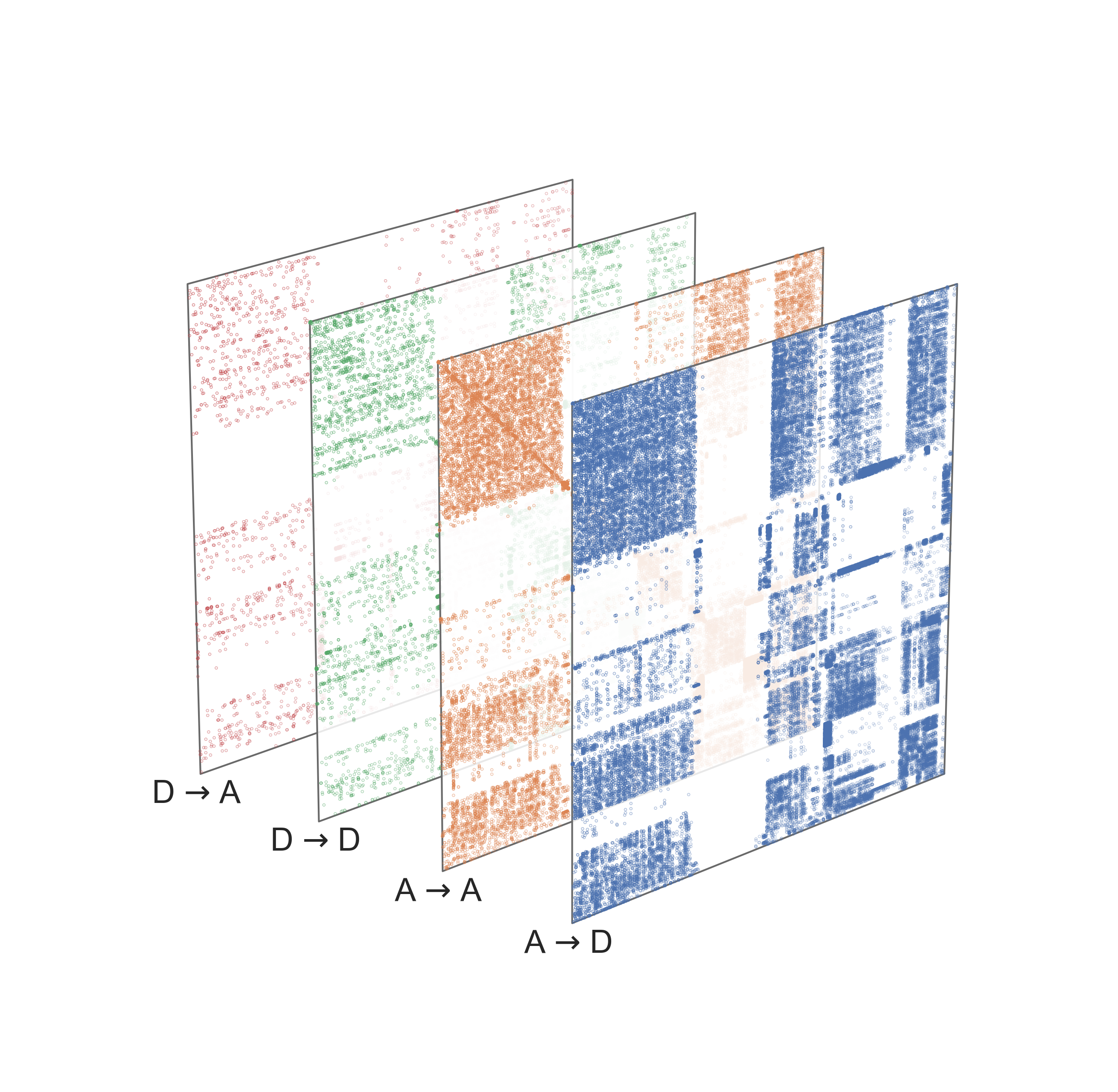
Fig. 21 Example of a multiple-layered network (multigraph) from the Drosophila larva brain connectome.

Or, we may have networks which arise from the same process, but at different timepoints.

Regardless of the data, it is common to want to:

• Compare the role/structure of each node across networks, or

• Generate a single embedding which summarizes the property of each node, regardless of which network it came from, or

• Quantitatively compare the networks themselves

Each of these tasks (and many others) can benefit from doing network embeddings which somehow deal with multiple networks. We’ll discuss a few approaches and considerations below, mainly for the spectral methods.

Note

Many other approaches for doing multiple network embeddings exist, including for some of the neural network approaches.

Do a couple of spectral embeddings

Let’s say we have two networks. We wish to come up with an embedding for each node in each network. Since we’ve already learned about techniques for network embedding, why not just apply these techniques separately to each network, and compare the results?

import networkx as nx
import pandas as pd
from pathlib import Path
from graspologic.utils import symmetrize


DATA_PATH = Path("networks-course/data")


def load_matched(side="left"):
    side = side.lower()
    dir = DATA_PATH / "processed_maggot"
    g = nx.read_edgelist(
        dir / f"matched_{side}_edgelist.csv",
        create_using=nx.DiGraph,
        delimiter=",",
        nodetype=int,
    )
    nodes = pd.read_csv(dir / f"matched_{side}_nodes.csv", index_col=0)
    adj = nx.to_numpy_array(g, nodelist=nodes.index)
    return adj, nodes


left_adj, left_nodes = load_matched("left")
right_adj, right_nodes = load_matched("right")
left_adj = symmetrize(left_adj)
right_adj = symmetrize(right_adj)

from graspologic.embed import AdjacencySpectralEmbed

ase = AdjacencySpectralEmbed(n_components=8)
X_left = ase.fit_transform(left_adj)
X_right = ase.fit_transform(right_adj)

import numpy as np
from graspologic.plot import pairplot

X_both = np.concatenate((X_left, X_right), axis=0)
labels = np.array(len(X_left) * ["Left"] + len(X_right) * ["Right"])

pairplot(X_both[:, :4], labels, legend_name="Side", title="Latent position estimates")

<seaborn.axisgrid.PairGrid at 0x12e684c10>

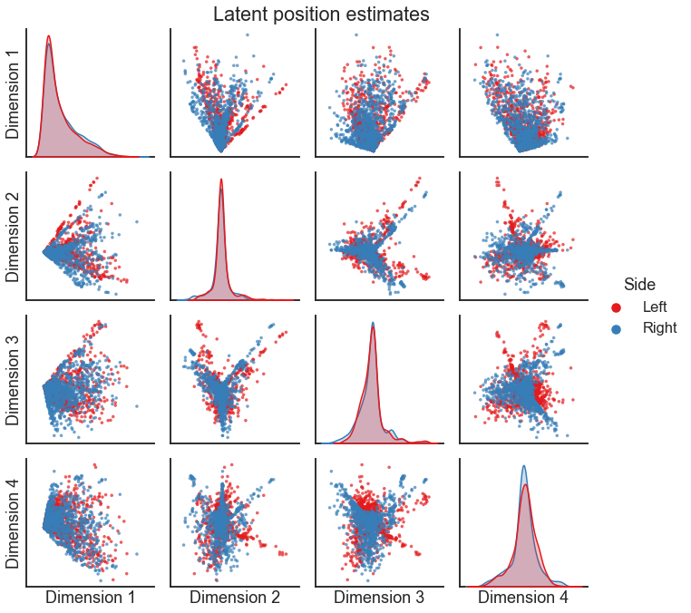
Question

Based on this plot, would you say that these networks are similar? Why or why not?

Do you notice anything about the relationship of one embedding with regard to the other?

Orthogonal nonidentifiability

Earlier in the course, we discussed a model with a nonidentifiability in its parameters. As a reminder, this just means that we have some flexibility in the parameters we use which gives us the same model behavior. Can this arise for the RDPG model, which is the motivation behind doing ASE? Let’s have a look.

Remember that for the RDPG, we are using the model of \(A\) being sampled from a probability matrix, \(P\). \(P\) has the structure

\[P = XX^T\]

for an undirected network, or for a directed network,

\[P = XY^T\]

How can a nonidentifiability pop up here? Note that an orthogonal matrix \(W\) is one such that

\[W W^T = W^T W = I\]

Intuitively, these orthogonal matrices represent rotations and reflections in our \(d\)-dimensional space. They are often called isometric transformations of the space, because they preserve all interpoint distances.

import matplotlib.pyplot as plt
import seaborn as sns

sns.set_context("talk")

X = np.array([[0.2, 0.5], [0.1, 0.6], [0.7, 0.05]])

fig, axs = plt.subplots(1, 2, figsize=(12, 6))

ax = axs[0]
for row in X:
    ax.plot([0.0, row[0]], [0.0, row[1]], linewidth=3)

ax.axis("off")
ax.axvline(0, color="black", linewidth=1)
ax.axhline(0, color="black", linewidth=1)
ax.set_title(r"Original positions ($X$)")

from scipy.stats import ortho_group

np.random.seed(888)
W = ortho_group.rvs(2)

Z = X @ W

ax = axs[1]
for row in Z:
    ax.plot([0.0, row[0]], [0.0, row[1]], linewidth=3)

ax.axis("off")
ax.axvline(0, color="black", linewidth=1)
ax.axhline(0, color="black", linewidth=1)
ax.set_title(r"Transformed positions ($X W$)")

Text(0.5, 1.0, 'Transformed positions ($X W$)')

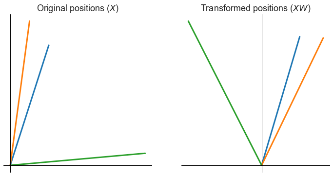
Note that the distances between all points is preserved.

Question

Can you think of another set of latent positions, say \(Z\), such that or probability matrix \(P = XX^T = ZZ^T\), but \(Z \neq X\)?

Hint: where can you insert some orthogonal matrices into the formula \(P = XX^T\) such that the matrix \(P\) is unchanged?

Note what this means for our embeddings:

W = ortho_group.rvs(X_left.shape[1])
X_left_new = X_left @ W
P1 = X_left @ X_left.T
P2 = X_left_new @ X_left_new.T

np.isclose(P1, P2).all()

True

We have just found two sets of latent positions which are equally valid - but note that there are an infinite number of orthogonal transformations.

Orthogonal procrustes problem

In practice, how can we resolve this issue? Let’s say we have these two sets of latent positions, \(X^{(1)}\) and \(X^{(2)} W\), and want to somehow compare them on equal footing. What we can do is try to uncover a orthogonal transformation of one set of latent positions with regard to the other, e.g.

\[X^{(1)} \text{ vs. } X^{(2)} W\]

for some \(W\).

Question

What would be a good way to measure the distance between \(X^{(1)}\) and \(X^{(2)} W\)?

We arrive at the problem

\[\min_{W: WW^T=W^TW=I} \|X^{(1)} - X^{(2)} W\|_F\]

This is a very old and famous problem known as the orthogonal Procrustes problem, and it has an exact solution (fun fact: the solution uses the SVD).

We can apply the Procrustes solution using scipy.linalg.orthogonal_procrustes or a wrapper in graspologic, the OrthogonalProcrustes class.

from graspologic.align import OrthogonalProcrustes

op = OrthogonalProcrustes()
X_right_pred = op.fit_transform(X_right, X_left)

X_both = np.concatenate((X_left, X_right_pred), axis=0)

pairplot(
    X_both[:, :4],
    labels,
    legend_name="Side",
    title="Latent position estimates (mapped)",
)

<seaborn.axisgrid.PairGrid at 0x134f0abe0>

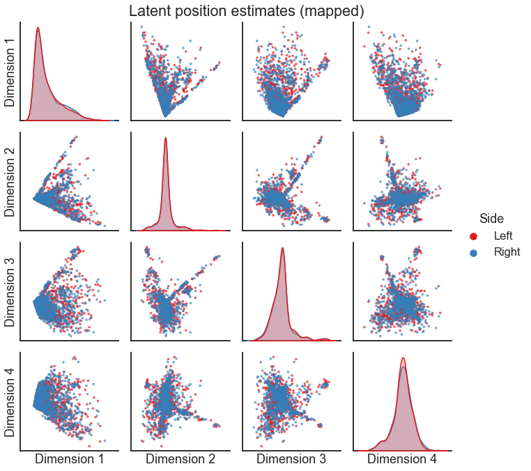
Question

Looking at these embeddings, would you say these networks are similar or different, at least at a high level?

Considerations

Question

Does the order of nodes in \(X^{(2)}\) matter? What does it represent?

rng = np.random.default_rng(88)
perm_inds = rng.permutation(len(X_right))
op = OrthogonalProcrustes()
X_right_pred = op.fit_transform(X_right[perm_inds], X_left)

X_both = np.concatenate((X_left, X_right_pred), axis=0)

pairplot(
    X_both[:, :4],
    labels,
    legend_name="Side",
    title="Latent position estimates (shuffled, mapped)",
)

<seaborn.axisgrid.PairGrid at 0x137e3b0d0>

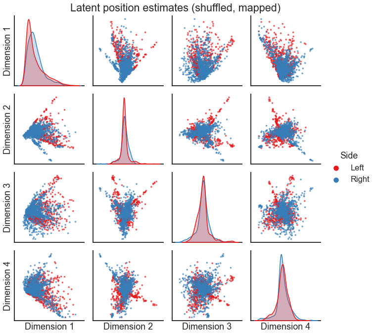
Note

The orthogonal Procrustes solution only works for pairs of networks where we know the mapping between node \(i\), graph 1 and node \(i\), graph 2. As a consequence, this would only work if the networks have the same size.

Note that we can use something called SeedlessProcrustes in graspologic if we had two networks of different sizes or where the mapping between nodes is unknown. There is more information about this method, as well as alignments in general, in the align tutorials.

Warning

The dimensionality of the embedding can have a huge effect on the quality of the alignment (for reasons I won’t go into here, but talk about in a forthcoming paper). I always recommend that you try a range of dimensionalities, and look at the embeddings after aligning them.

Omnibus Embedding

The method described above (basically just doing ASE twice) is a totally valid way of attacking this multiple network embedding problem, though it has many caveats. In practice, we often want to do multiple network embeddings without dealing with this alignment issue. For matched networks, we can use a technique called the Omnibus embedding (Omni, for short).

The algorithm itself is pretty simple. We essentially construct a larger matrix (described in the figure below) which is constructed from each of the individual adjacency matrices. We then decompose that larger matrix \(M\) using the same process as ASE. Because this embedding is done in one stage (rather than one for each network) we no longer have the same issue with the nonidentifiability above, so we no longer have to worry about aligning our embeddings between networks.

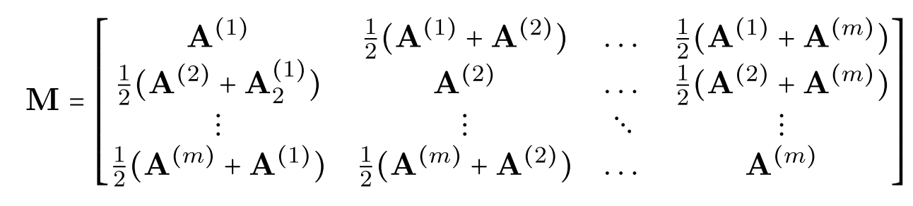
Fig. 22 Construction of the matrix \(M\) which is then decomposed using the SVD in the Omnibus embedding. Figure from Athreya et al. [1].

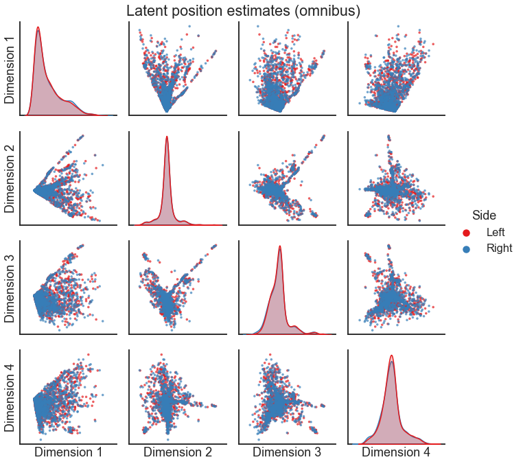
from graspologic.embed import OmnibusEmbed

omni = OmnibusEmbed(n_components=4)
X_left, X_right = omni.fit_transform([left_adj, right_adj])

X_both = np.concatenate((X_left, X_right), axis=0)

pairplot(
    X_both, labels, legend_name="Side", title="Latent position estimates (omnibus)"
)

<seaborn.axisgrid.PairGrid at 0x13807bd00>

Multiple ASE

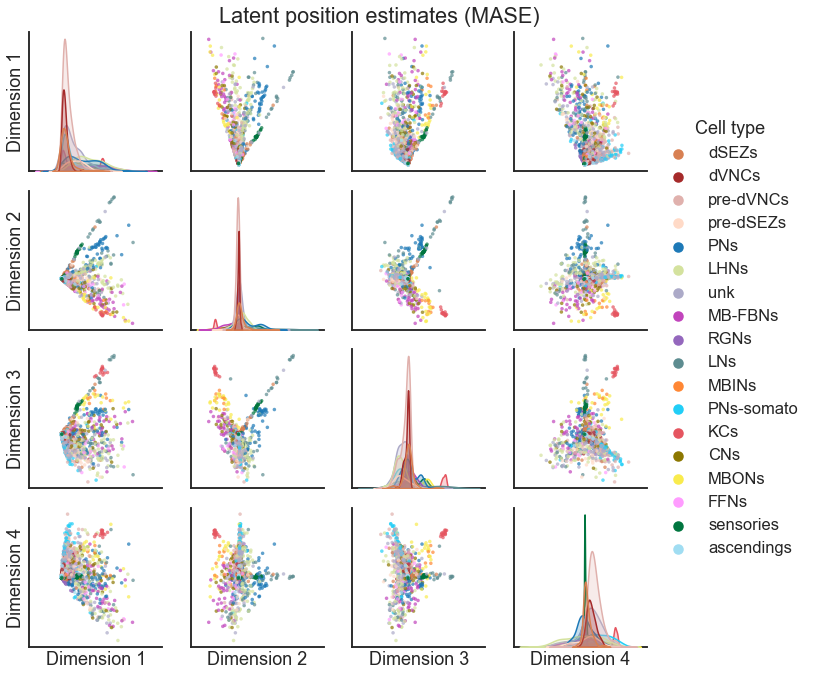
Sometimes, we aren’t as interested in having a representation for each node in each graph - perhaps we don’t care about what is different between networks, and we are interested in grouping nodes based on their shared structure across many different networks. An algorithm called multiple adjacency spectral embedding (MASE) introduced in Arroyo et al. [2] can be used for this task.

I won’t go into all the details of the algorithm, though I believe you all could understand it based on what we’ve talked about in this course. However, I’ll say that this algorithm is associated with a model, where we model the probability matrix for graph \(k\) as

\[P^{(k)} = V R^{(k)} V^T\]

Note that there is no superscript on the \(V\) - these are node-wise representations which are shared across all of the networks. You can think of this as one embedding for each node in the network, but we got it using all of the networks to form this representation. The \(R^{(k)}\) matrices, sometimes called the “score” matrices, are able of representing how each network is (potentially) different.

Using MASE is easy in graspologic. Here, we apply it to form a latent position estimate for each node pair

import json
from graspologic.embed import MultipleASE

with open(DATA_PATH / "processed_maggot/simple_color_map.json", "r") as f:
    palette = json.load(f)

mase = MultipleASE(n_components=4)
X_joint = mase.fit_transform([left_adj, right_adj])

node_labels = left_nodes["simple_group"].values

pairplot(
    X_joint,
    node_labels,
    legend_name="Cell type",
    title="Latent position estimates (MASE)",
    palette=palette,
)

<seaborn.axisgrid.PairGrid at 0x1387248b0>

Note

The MASE algorithm also has a method for extracting a representation per network. In graspologic, these can be accessed using the .score_ attribute of the fitted object. More details can be found in the MASE tutorial.

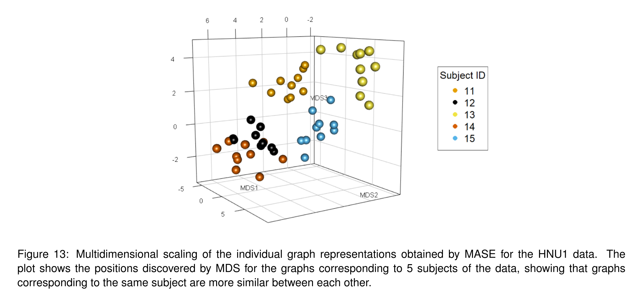
Fig. 23 Example of extracting a per-graph representation from the MASE algorithm. Figure from Arroyo et al. [2].

Representations for each network

The following example comes from the graspologic tutorial on multiscale comparative connectomics, which is based on Gopalakrishnan et al. [3]. The data comes from Wang et al. [4].

Below, we load in 32 networks - these networks come from MRI scans of mice brains, and these mouse came from one of 4 different genotypes. There are 8 mice from each genotype.

from graspologic.datasets import load_mice

# Load the full mouse dataset
mice = load_mice()

# Stack all adjacency matrices in a 3D numpy array
graphs = np.array(mice.graphs)
graphs.shape

(32, 332, 332)

As before, we can use the Omnibus embedding to construct an embedding for each network in the same space, without having to do any alignment.

Note

You could absolutely try doing this step with any of the other embedding methods that we talked about!

# Jointly embed graphs using omnibus embedding
embedder = OmnibusEmbed(n_elbows=3)
omni_embedding = embedder.fit_transform(graphs)
print(omni_embedding.shape)

(32, 332, 9)

Now, we have an embedding for each node in each network, and we know that these nodes are matched across networks. To measure the difference between two networks, then, we can do something like

\[d(k, l) = \|X^{(k)} - X^{(l)}\|_F\]

Now, we can do this for each \((k, l)\) pair of networks, and create a distance matrix, \(D\).

\[D_{kl} = d(k, l)\]

dissimilarity_matrix = np.zeros((len(graphs), len(graphs)))

# note: this is a slow way of doing this, but also the most clear to understand.
for i, embedding1 in enumerate(omni_embedding):
    for j, embedding2 in enumerate(omni_embedding):
        dist = np.linalg.norm(embedding1 - embedding2, ord="fro")
        dissimilarity_matrix[i, j] = dist

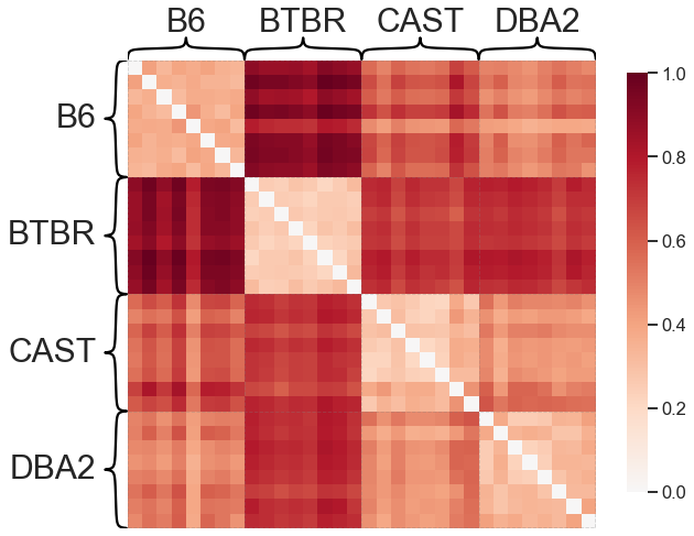
What does this matrix of dissimilarities look like?

from graspologic.plot import heatmap

scaled_dissimilarity = dissimilarity_matrix / np.max(dissimilarity_matrix)

_ = heatmap(scaled_dissimilarity, context="talk", inner_hier_labels=mice.labels)

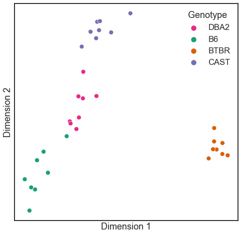
A technique called classical multidimensional scaling can be used to embed a matrix of distances or dissimilarities, much like we have been discussing the embedding of networks.

In graspologic, the ClassicalMDS class can operate on a dissimilarity matrix directly as we do below using the dissimilarity='precomputed' flag. You can also directly pass in omni_embedding, if you wanted.

from graspologic.embed import ClassicalMDS
from graspologic.plot import heatmap

# Further reduce embedding dimensionality using cMDS
cmds = ClassicalMDS(n_components=2, dissimilarity="precomputed")
cmds_embedding = cmds.fit_transform(scaled_dissimilarity)
cmds_embedding = pd.DataFrame(cmds_embedding, columns=["Dimension 1", "Dimension 2"])
cmds_embedding["Genotype"] = mice.labels

palette = {"DBA2": "#e7298a", "B6": "#1b9e77", "BTBR": "#d95f02", "CAST": "#7570b3"}

fig, ax = plt.subplots(1, 1, figsize=(8, 8))
sns.scatterplot(
    x="Dimension 1",
    y="Dimension 2",
    hue="Genotype",
    data=cmds_embedding,
    palette=palette,
    ax=ax,
)
ax.set_xticks([])
_ = ax.set_yticks([])

What if we hadn’t known the genotype labels ahead of time, and wanted to cluster the networks into meaningful groups? We can just run your favorite clustering algorithm, either on the set of points learned by classical multidimensional scaling, or by clustering directly on the dissimilarity matrix as I do below.

from scipy.cluster import hierarchy
from scipy.spatial.distance import squareform

Z = hierarchy.linkage(squareform(scaled_dissimilarity), method="single")

network_colors = np.vectorize(palette.get)(mice.labels)

clustergrid = sns.clustermap(
    scaled_dissimilarity,
    row_linkage=Z,
    col_linkage=Z,
    row_colors=network_colors,
    col_colors=network_colors,
    cmap="RdBu_r",
    center=0,
    xticklabels=False,
    yticklabels=False,
)

# label the colorbar
clustergrid.ax_cbar.set_title("Dissimilarity", pad=15)

# label one of the object color labels
col_ax = clustergrid.ax_col_colors
col_ax.set_yticks([0.5])
_ = col_ax.set_yticklabels(["Genotype"], va="center")

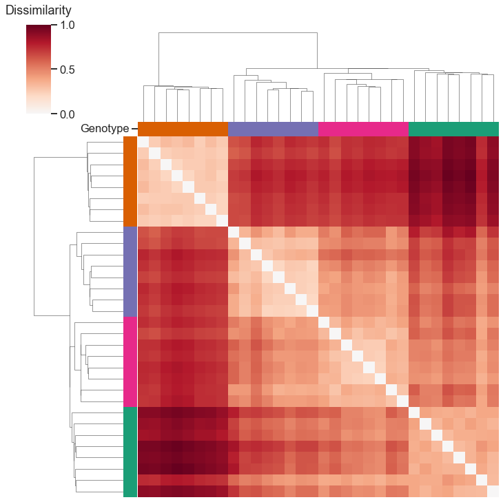
With this representation that we learned from our network embeddings, our clustering exactly recovered the genotype labels!

References

[1]

Avanti Athreya, Donniell E Fishkind, Minh Tang, Carey E Priebe, Youngser Park, Joshua T Vogelstein, Keith Levin, Vince Lyzinski, and Yichen Qin. Statistical inference on random dot product graphs: a survey. The Journal of Machine Learning Research, 18(1):8393–8484, 2017.

[2] (1,2)

Jesús Arroyo, Avanti Athreya, Joshua Cape, Guodong Chen, Carey E Priebe, and Joshua T Vogelstein. Inference for multiple heterogeneous networks with a common invariant subspace. Journal of Machine Learning Research, 22(142):1–49, 2021.

[3]

Vivek Gopalakrishnan, Jaewon Chung, Eric Bridgeford, Benjamin D Pedigo, Jesús Arroyo, Lucy Upchurch, G Allan Johnson, Nian Wang, Youngser Park, Carey E Priebe, and others. Multiscale comparative connectomics. arXiv preprint arXiv:2011.14990, 2020.

[4]

Nian Wang, Robert J Anderson, David G Ashbrook, Vivek Gopalakrishnan, Youngser Park, Carey E Priebe, Yi Qi, Rick Laoprasert, Joshua T Vogelstein, Robert W Williams, and others. Variability and heritability of mouse brain structure: microscopic mri atlases and connectomes for diverse strains. NeuroImage, 222:117274, 2020.