Random network models

This notebook on random network models is adapted from the graspoloigc tutorial on the same topic.

You may also be interested in a similar section in Hands-on Network Machine Learning with Scikit-Learn and Graspologic.

Why use random network models?

There are a few different reasons one might want to use a statistical network model.

First, these models can be a concise, mathematical way of formalizing a conception of the process involved in generating a network.

Second, we may want to use a simple model which captures some aspects of our network’s structure to compare to - for instance, how does the community structure of a network we observe compare to a network generated from a Random Dot Product Graph (more on this later)?

Third, these models are often useful for motivating or proving properties of how our algorithms perform on data.

Fourth, these models (and their parameters) can be a lens through which we can compare networks.

I note that these are mostly my opinions, and other people’s reasons for using statistical network models might differ. For whatever the reason, these models come up in research a ton. Let’s look at a few of these models below.

Load some data from graspologic

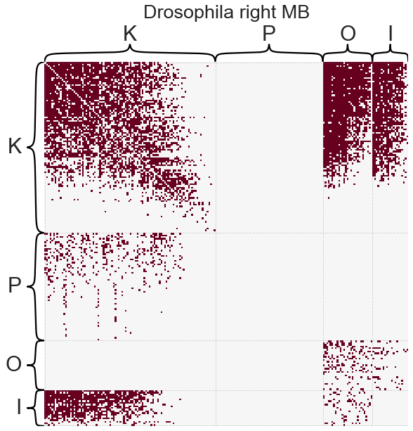
For this example we will use the Drosophila melanogaster larva right mushroom body connectome from Eichler et al. 2017. Here we will consider a binarized and directed version of the graph. Note that I will make this graph unweighted, because most statistical network models are concerned with binary networks.

import numpy as np
from graspologic.datasets import load_drosophila_right
from graspologic.plot import heatmap
from graspologic.utils import binarize

adj, labels = load_drosophila_right(return_labels=True)
adj = binarize(adj)

degrees = adj.sum(axis=0) + adj.sum(axis=1)
sort_inds = np.argsort(-degrees)
adj = adj[sort_inds][:, sort_inds]
labels = labels[sort_inds]

_ = heatmap(
    adj,
    inner_hier_labels=labels,
    title="Drosophila right MB",
    font_scale=1.5,
    sort_nodes=False,
    cbar=False,
)

Notation

\(n\) - the number of nodes in the graph

\(A\) - \(n \times n\) adjacency matrix

\(P\) - \(n \times n\) matrix of probabilities

Independent edge models

Many statistical network models fall under the umbrella of independent edge random networks, sometimes called the Inhomogeneous Erdos-Renyi (IER) model. Under this model, the elements of the network’s adjacency matrix \(A\) are sampled independently from a Bernoulli distribution:

\[A_{ij} \sim Bernoulli(P_{ij})\]

If \(n\) is the number of nodes, the matrix \(P\) is a \(n \times n\) matrix of probabilities with elements in \([0, 1]\). Depending on how the matrix \(P\) is constructed, we can create various different specific models. We next describe several of these choices. Note that for each model, we assume that there are no loops, or in other words the diagonal of the matrix \(P\) will always be set to zero.

For each graph model we will show:

• how the model is formulated

• how to fit the model using graspologic

• the \(P\) matrix that was fit by the model

• a single sample of a new network from the fit model

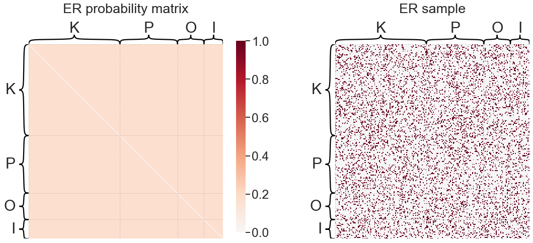
Erdos-Reyni (ER)

The Erdos-Reyni (ER) model is the simplest random graph model. We are interested in modeling the probability of an edge existing between any two nodes, \(i\) and \(j\). We denote this probability \(P_{ij}\). For the ER model:

\[P_{ij} = p\]

for any combination of \(i\) and \(j\).
This means that the one parameter \(p\) is the overall probability of connection for any two nodes.

from graspologic.models import EREstimator

er = EREstimator(directed=True, loops=False)
er.fit(adj)
print(f'ER "p" parameter: {er.p_}')


def plot_model_and_sample(estimator, name):
    fig, axs = plt.subplots(1, 2, figsize=(20, 10), sharey=True)
    heatmap(
        estimator.p_mat_,
        inner_hier_labels=labels,
        vmin=0,
        vmax=1,
        font_scale=1.5,
        title=f"{name} probability matrix",
        sort_nodes=False,
        ax=axs[0],
    )
    ax = heatmap(
        estimator.sample()[0],
        inner_hier_labels=labels,
        font_scale=1.5,
        title=f"{name} sample",
        sort_nodes=False,
        ax=axs[1],
    )
    fig.axes[5].remove()


plot_model_and_sample(er, "ER")

ER "p" parameter: 0.1661046088739007

networkx also has an ER sampler. Note the directed kwarg.

import networkx as nx

n = adj.shape[0]
p = er.p_

nx.erdos_renyi_graph(n=n, p=p, directed=True)

<networkx.classes.digraph.DiGraph at 0x141056280>

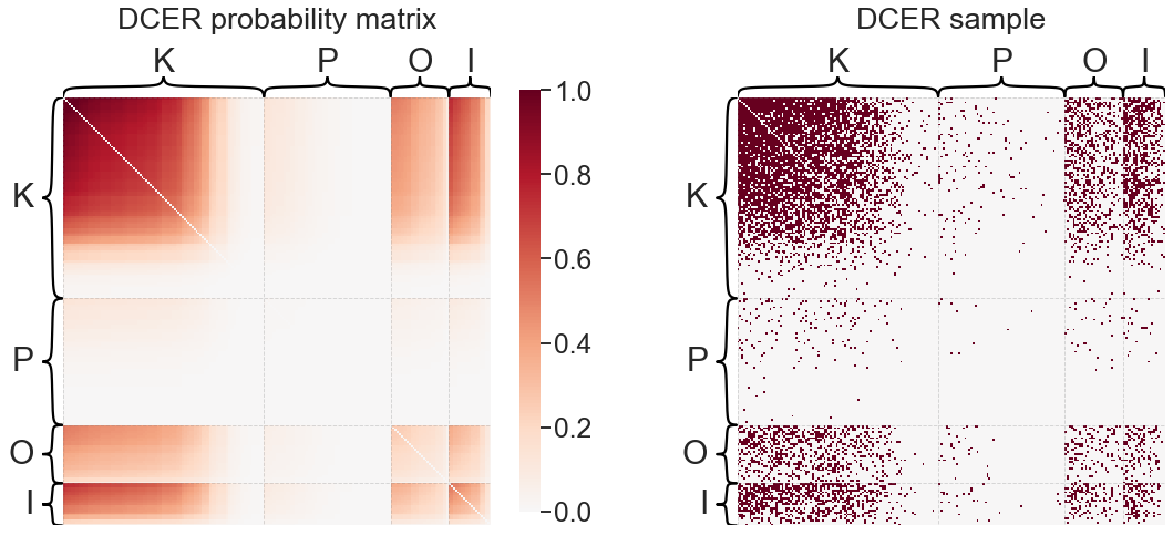
Degree-corrected Erdos-Reyni (DCER)

A slightly more complicated variant of the ER model is the degree-corrected Erdos-Reyni model (DCER). Here, there is still a global parameter \(p\) to specify relative connection probability between all edges. However, we add a promiscuity parameter \(\theta_i\) for each node \(i\) which specifies its expected degree relative to other nodes:

\[P_{ij} = \theta_i \theta_j p\]

so the probability of an edge from \(i\) to \(j\) is a function of the two nodes’ degree-correction parameters, and the overall probability of an edge in the graph.

Note

There is a commonly used network model called the configuration model which exactly specifies the degree sequence, and is usually sampled somewhat differently. We use the DCER term for consistency with the rest of these models, but note that this is very similar in spirit to a configuration model.

Note

This model has what is called a nonidentifiability this can be thought of as having some flexibility in the model parameters which has no effect on the model itself. We could multiply \(p\) by 2, and divide the vector \(\theta\) by 2, and have the same matrix \(P\). As an aside, nonidentifiabilities are important to consider when comparing parameters. Here, we just use the convention that \(\theta\) sum to 1, which gives \(p\) the interpretation as the expected number of edges.

from graspologic.models import DCEREstimator

dcer = DCEREstimator(directed=True, loops=False)
dcer.fit(adj)
print(f'DCER "p" parameter: {dcer.p_}')

plot_model_and_sample(dcer, "DCER")

DCER "p" parameter: 7536.0

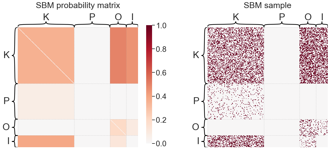
Stochastic block model (SBM)

Under the stochastic block model (SBM), each node is modeled as belonging to a block (sometimes called a community or group). The probability of node \(i\) connecting to node \(j\) is simply a function of the block membership of the two nodes. Let \(n\) be the number of nodes in the graph, then \(\tau\) is a length \(n\) vector which indicates the block membership of each node in the graph. Let \(K\) be the number of blocks, then \(B\) is a \(K \times K\) matrix of block-block connection probabilities.

\[P_{ij} = B_{\tau_i \tau_j}\]

from graspologic.models import SBMEstimator

sbme = SBMEstimator(directed=True, loops=False)
sbme.fit(adj, y=labels)
print('SBM "B" matrix:')
print(sbme.block_p_)

plot_model_and_sample(sbme, "SBM")

SBM "B" matrix:
[[0.         0.38333333 0.11986864 0.        ]
 [0.44571429 0.3584     0.49448276 0.        ]
 [0.09359606 0.         0.20095125 0.        ]
 [0.         0.07587302 0.         0.        ]]

Note

In the above, we had to pass in the group labels which told us which node belong to which group in the SBM. There is a huge body of work on how to infer which group every node belongs to, which we should talk about later in the course.

For now, just note that graspologic implements one simple method for inferring these labels if they are not passed in, but I would not trust this quick method without reviewing the results. graph-tool is also an excellent library which has some tools for inferring group membership, but this library has a bit of a learning curve.

networkx also has an SBM sampler.

sizes = [50, 75]  # size in each group
p = [[0.9, 0.1], [0.05, 0.6]]  # matrix of probabilities

nx.stochastic_block_model(sizes, p, directed=True)

<networkx.classes.digraph.DiGraph at 0x141d4d460>

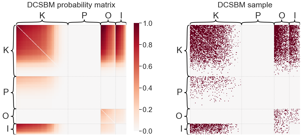
Degree-corrected stochastic block model (DCSBM)

Just as we could add a degree-correction term to the ER model, so too can we modify the stochastic block model to allow for heterogeneous expected degrees. This yields the degree-corrected stochastic block model. Again, we let \(\theta\) be a length \(n\) vector of degree correction parameters, and all other parameters remain as they were defined above for the SBM:

\[P_{ij} = \theta_i \theta_j B_{\tau_i, \tau_j}\]

Note that the matrix \(B\) may no longer represent true probabilities, because the addition of the \(\theta\) vectors introduces a multiplicative constant that can be absorbed into the elements of \(\theta\).

from graspologic.models import DCSBMEstimator

dcsbme = DCSBMEstimator(directed=True, loops=False)
dcsbme.fit(adj, y=labels)
print('DCSBM "B" matrix:')
print(dcsbme.block_p_)

plot_model_and_sample(dcsbme, "DCSBM")

DCSBM "B" matrix:
[[   0.  805.   73.    0.]
 [ 936. 3584. 1434.    0.]
 [  57.    0.  169.    0.]
 [   0.  478.    0.    0.]]

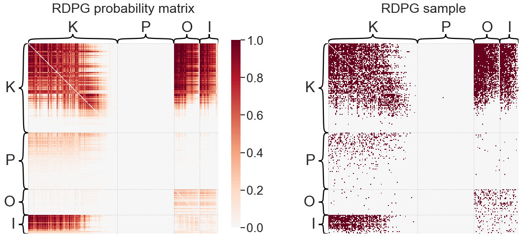
Random dot product graph (RDPG)

The random dot product graph model (RDPG) [1, 2] is a (relatively speaking) newer network model under the umbrella of latent position random graphs [3]. Under latent position models, each node has an associated, typically unobserved vector which is referred to as the latent position of that node. For the directed network case, we can allow each node to have associated “in” and “out” latent position vectors which may not be the same, with the former governing the nodes inputs and the latter governing its outputs. If \(x_i\) is the out latent position for node \(i\), and \(y_j\) the input latent position for node \(j\), then the probability of an edge between \(i\) and \(j\) is some function of these vectors:

\[P[A_{ij} = 1] = P_{ij} = f(x_i, y_j)\]

More specifically for the RDPG, the link function \(f\) is the dot product:

\[P[A_{ij} = 1] = P_{ij} = \langle x_i, y_j \rangle\]

The latent positions are thus restricted such that \(\langle x_i, y_j \rangle \in [0, 1]\) for all \((i,j)\) pairs. Under this definition, \(P\), the matrix of connection probabilities, can be written as \(P = XY^T\), where \(X \in \mathbb{R}^{n \times d}\) is a matrix where each row \(i\) is the out latent position of node \(i\), and likewise for \(Y\) and the in latent positions.

Question

Imagine that the out and in latent positions are the same (\(x_i = y_i\)). Describe a restriction on the latent positions (say, a region of space) such that all probabilities are well defined.

Hint: what would the restriction be when \(d=1\)? When \(d=2\)?

In practical applications, we never observe the latent positions in \(X\) and \(Y\) - they must be estimated from the observed network, \(A\). Fortunately, this can be done via an established technique known as adjacency spectral embedding (ASE) [1], which was recently shown to be a consistent estimator of these latent positions. We’ll discuss this more when we talk about network embeddings.

from graspologic.models import RDPGEstimator

rdpge = RDPGEstimator(loops=False)
rdpge.fit(adj, y=labels)

plot_model_and_sample(rdpge, "RDPG")

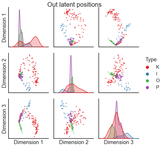
For the RDPG, looking at the model parameters can be more challenging, since in this case they are a \(d\)-dimensional vector for each node. We can access the estimated \(X\) and \(Y\) matrices:

X = rdpge.latent_[0]
Y = rdpge.latent_[1]

print(X.shape)
print(Y.shape)

(213, 3)
(213, 3)

One way to visualize these multidimensional sets of vectors (each row of \(X\) and \(Y\) is a vector which corresponds to a node) is to use graspologic’s pairplot, which itself is just a wrapper around seaborn’s pairplot.

from graspologic.plot import pairplot

pairplot(X, labels=labels, title="Out latent positions")

<seaborn.axisgrid.PairGrid at 0x142425640>

Compare all of the models on this dataset

import matplotlib as mpl
import matplotlib.pyplot as plt
import seaborn as sns
from matplotlib import cm

fig, axs = plt.subplots(2, 3, figsize=(20, 16))

sns.set_context("talk")
# colormapping
cmap = cm.get_cmap("RdBu_r")

center = 0
vmin = 0
vmax = 1
norm = mpl.colors.Normalize(0, 1)
cc = np.linspace(0.5, 1, 256)
cmap = mpl.colors.ListedColormap(cmap(cc))

# heatmapping
heatmap_kws = dict(
    inner_hier_labels=labels,
    vmin=0,
    vmax=1,
    cbar=False,
    cmap=cmap,
    center=None,
    hier_label_fontsize=20,
    title_pad=45,
    font_scale=1.6,
    sort_nodes=True,
)

models = [rdpge, dcsbme, dcer, sbme, er]
model_names = ["RDPG", "DCSBM", "DCER", "SBM", "ER"]

heatmap(adj, ax=axs[0][0], title="Data", **heatmap_kws)
heatmap(models[0].p_mat_, ax=axs[0][1], title=model_names[0], **heatmap_kws)
heatmap(models[1].p_mat_, ax=axs[0][2], title=model_names[1], **heatmap_kws)
heatmap(models[2].p_mat_, ax=axs[1][0], title=model_names[2], **heatmap_kws)
heatmap(models[3].p_mat_, ax=axs[1][1], title=model_names[3], **heatmap_kws)
heatmap(models[4].p_mat_, ax=axs[1][2], title=model_names[4], **heatmap_kws)


# add colorbar
sm = plt.cm.ScalarMappable(cmap=cmap, norm=norm)
sm.set_array(dcsbme.p_mat_)
cbar = fig.colorbar(
    sm,
    ax=axs,
    orientation="horizontal",
    pad=0.04,
    shrink=0.75,
    fraction=0.08,
    drawedges=False,
)

cbar.ax.set_ylabel("Edge probability", rotation=0, ha="right", va="center")
cbar.ax.yaxis.set_visible(True)

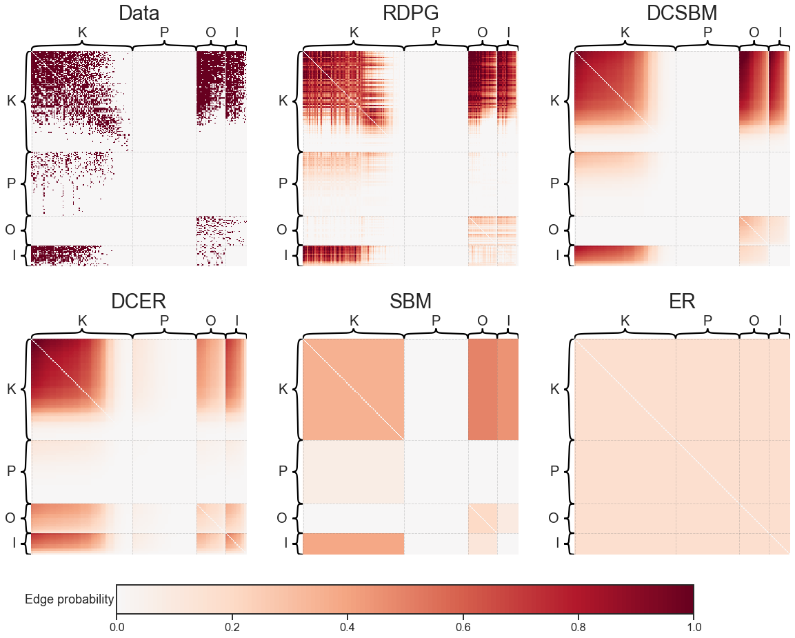
Relationships among these models

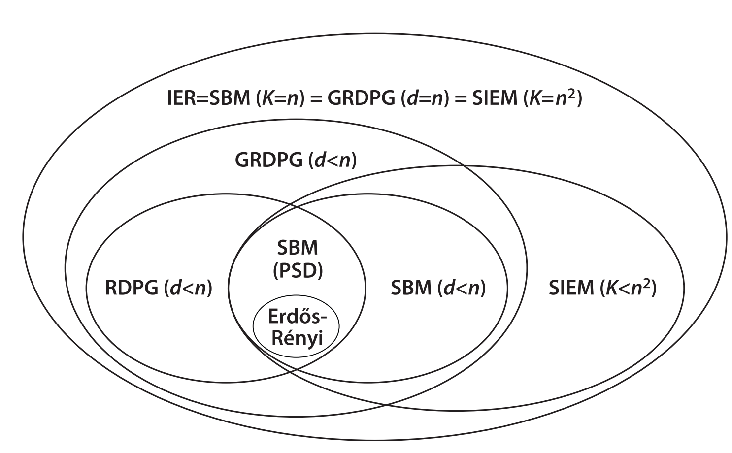
Fig. 4 Relationships among independent edge models (some not mentioned here). Figure from Chung et al. [4].

Question

When can an SBM also be considered an ER model?

Question

When can an SBM be considered a DCSBM?

Question

When can an RDPG be considered a SBM?

Question

When can an RDPG be considered a DCSBM?

Hint: have a look at the last plot in this notebook.

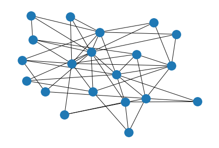
Barabasi-Albert model

Here, we quickly give one example of a non-independent edge model.

The Barabasi-Albert (BA) model is a model based on the idea of preferential attachment, sometimes called “rich-get-richer” phenomena.

In contrast to the previous models, the BA model is based on a time-evolving process. Put simply, the idea is that nodes with higher degrees at time \(t\) are more likely to make new edges at time \(t+1\).

Generating this model follows a fairly simple process. First, at time \(t=0\), we start with \(n_0\) nodes in some pre-specified configuration. At time \(t=1\), we add one new node which makes \(m\) edges to the existing network. The probability \(p_i\) that this new node is connected to node \(i\) is simply

\[ p_i = \frac{k_i}{\sum_j k_j} \]

where \(k_i\) is the degree of node \(i\). This formula just says to connect in proportion to the degree of existing nodes.

Then, this process is repeated until the desired number of nodes is reached.

networkx has a function barabasi_albert_graph for creating networks this way.

n = 20  # number of desired nodes
m = 3  # number of edges each node should make

g = nx.barabasi_albert_graph(n, m)

nx.draw_kamada_kawai(g)

Other models

Many other network models have been described which we haven’t had time to cover here:

• Watts-Strogatz model for reproducing so-called “small-world” properties of many real networks, wherein there are relatively short paths among any pair of nodes even in a large network.

• Configuration model which exactly replicated a given degree distribution.

“Bespoke” models

Your network model does not just have to rely on the network itself, but can actually include other factors relevant to the application domain. For instance, one could use the spatial location of brain regions as part of a network model of the brain.

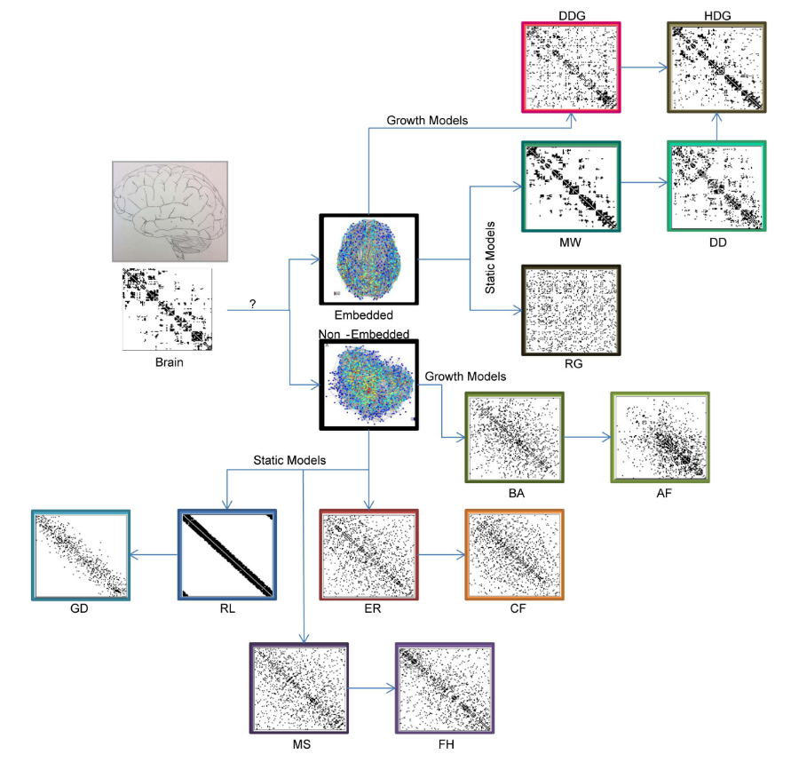
Fig. 5 Example models of brain connectivity. Figure from Klimm et al. [5]

References

[1] (1,2)

Avanti Athreya, Donniell E Fishkind, Minh Tang, Carey E Priebe, Youngser Park, Joshua T Vogelstein, Keith Levin, Vince Lyzinski, and Yichen Qin. Statistical inference on random dot product graphs: a survey. The Journal of Machine Learning Research, 18(1):8393–8484, 2017.

[2]

Stephen J Young and Edward R Scheinerman. Random dot product graph models for social networks. In International Workshop on Algorithms and Models for the Web-Graph, 138–149. Springer, 2007.

[3]

Peter D Hoff, Adrian E Raftery, and Mark S Handcock. Latent space approaches to social network analysis. Journal of the american Statistical association, 97(460):1090–1098, 2002.

[4]

Jaewon Chung, Eric Bridgeford, Jesús Arroyo, Benjamin D Pedigo, Ali Saad-Eldin, Vivek Gopalakrishnan, Liang Xiang, Carey E Priebe, and Joshua T Vogelstein. Statistical connectomics. Annual Review of Statistics and Its Application, 8:463–492, 2021.

[5]

Florian Klimm, Danielle S Bassett, Jean M Carlson, and Peter J Mucha. Resolving structural variability in network models and the brain. PLoS computational biology, 10(3):e1003491, 2014.