Plotting larger networks#
Load the data#
The data can be found here.
Simply download and make a networks-course/data/hemibrain folder to run this locally.
import time
from pathlib import Path
import pandas as pd
import networkx as nx
import numpy as np
from scipy.sparse import csr_array

t0 = time.time()


data_path = Path("networks-course/data/hemibrain")

neuron_file = "traced-neurons.csv"
edgelist_file = "traced-total-connections.csv"

edgelist_df = pd.read_csv(data_path / edgelist_file)

g = nx.from_pandas_edgelist(
    edgelist_df,
    source="bodyId_pre",
    target="bodyId_post",
    edge_attr="weight",
    create_using=nx.DiGraph,
)
Create an adjacency matrix, sorted by a specified nodelist.
nodelist = list(g.nodes)
adj = nx.to_scipy_sparse_array(g, nodelist=nodelist)
Generating colors for each node#
It is common to color nodes by the output of some community detection algorithm. Note that I need to symmetrize the network to make Leiden work.
from graspologic.partition import leiden

currtime = time.time()
sym_adj = adj + adj.T
out = leiden(sym_adj)
print(f"{time.time() - currtime:.3f} seconds elapsed.")
166.856 seconds elapsed.
The output is a dictionary mapping node IDs to community IDs. In this case the node IDs are just integers 0 - n-1, since we input an adjacency matrix (which has no other labeling).
print(type(out))
<class 'dict'>
It turns out that the conversion of the sparse adjacency matrix to a graph format that
Leiden can use is the slowest part of this process. So we can speed it up by just
going straight from the NetworkX graph. Note that to_undirected() in NetworkX simply
chooses an edge at random if there are multiple edges between two nodes, so we use
this symmetrizing function instead.
def symmetrze_nx(g):
    """Leiden requires a symmetric/undirected graph. This converts a directed graph to
    undirected just for this community detection step"""
    sym_g = nx.Graph()
    for source, target, weight in g.edges.data("weight"):
        if sym_g.has_edge(source, target):
            sym_g[source][target]["weight"] = (
                sym_g[source][target]["weight"] + weight * 0.5
            )
        else:
            sym_g.add_edge(source, target, weight=weight * 0.5)
    return sym_g


currtime = time.time()
sym_g = symmetrze_nx(g)
out2 = leiden(sym_g)
print(f"{time.time() - currtime:.3f} seconds elapsed.")
21.526 seconds elapsed.
node_df = pd.Series(out2)
node_df.index.name = "node_id"
node_df.name = "community"
node_df = node_df.to_frame()
node_df
| community | |
|---|---|
| node_id | |
| 911129339 | 4 |
| 450302778 | 3 |
| 5813049438 | 1 |
| 362701895 | 0 |
| 770249286 | 5 |
| ... | ... |
| 1008399765 | 5 |
| 915951662 | 2 |
| 549226277 | 0 |
| 1077424293 | 4 |
| 1319591242 | 6 |
21733 rows × 1 columns
node_df["community"].value_counts()
5    5864
6    4203
3    3034
1    2996
2    2390
0    2320
4     926
Name: community, dtype: int64
Note
If you want more or fewer communities, you can play with the resolution parameter in
Leiden. You can also consider plotting colors for only the most popular 10 or 20
communities.
Below I create a palette (dictionary from community to color) using the
graspologic colors, but you can also use anything in matplotlib or seaborn (see
here for more info).
from graspologic.layouts.colors import _get_colors

# TODO this is a bit buried in graspologic, should expose it more explicitly
colors = _get_colors(True, None)["nominal"]

palette = dict(zip(node_df["community"].unique(), colors))
Node sizes#
Its also common to have the size of each node in the layout relate to the number or strength of connections it makes.
Here I remake the adjacency matrix just to make sure it is sorted the same as node_df.
nodelist = node_df.index
adj = nx.to_scipy_sparse_array(g, nodelist=nodelist)
node_df["strength"] = adj.sum(axis=1) + adj.sum(axis=0)
node_df['rank_strength'] = node_df['strength'].rank(method='dense')
Positioning each node#
There are many ways to position each node in a graph. Here I use a spectral embedding followed by UMAP, a nonlinear dimensionality reduction technique.
from graspologic.embed import LaplacianSpectralEmbed
from graspologic.utils import pass_to_ranks

ptr_adj = pass_to_ranks(adj)

currtime = time.time()
lse = LaplacianSpectralEmbed(n_components=32, concat=True)
lse_embedding = lse.fit_transform(adj)
print(f"{time.time() - currtime:.3f} seconds elapsed.")
2.507 seconds elapsed.
Note that the parameters below can make a big difference in the final layout. These are some reasonable defaults.
from umap import UMAP

currtime = time.time()
n_components = 32
n_neighbors = 32
min_dist = 0.8
metric = "cosine"
umap = UMAP(
    n_components=2,
    n_neighbors=n_neighbors,
    min_dist=min_dist,
    metric=metric,
)
umap_embedding = umap.fit_transform(lse_embedding)

print(f"{time.time() - currtime:.3f} seconds elapsed.")
26.661 seconds elapsed.
node_df["x"] = umap_embedding[:, 0]
node_df["y"] = umap_embedding[:, 1]
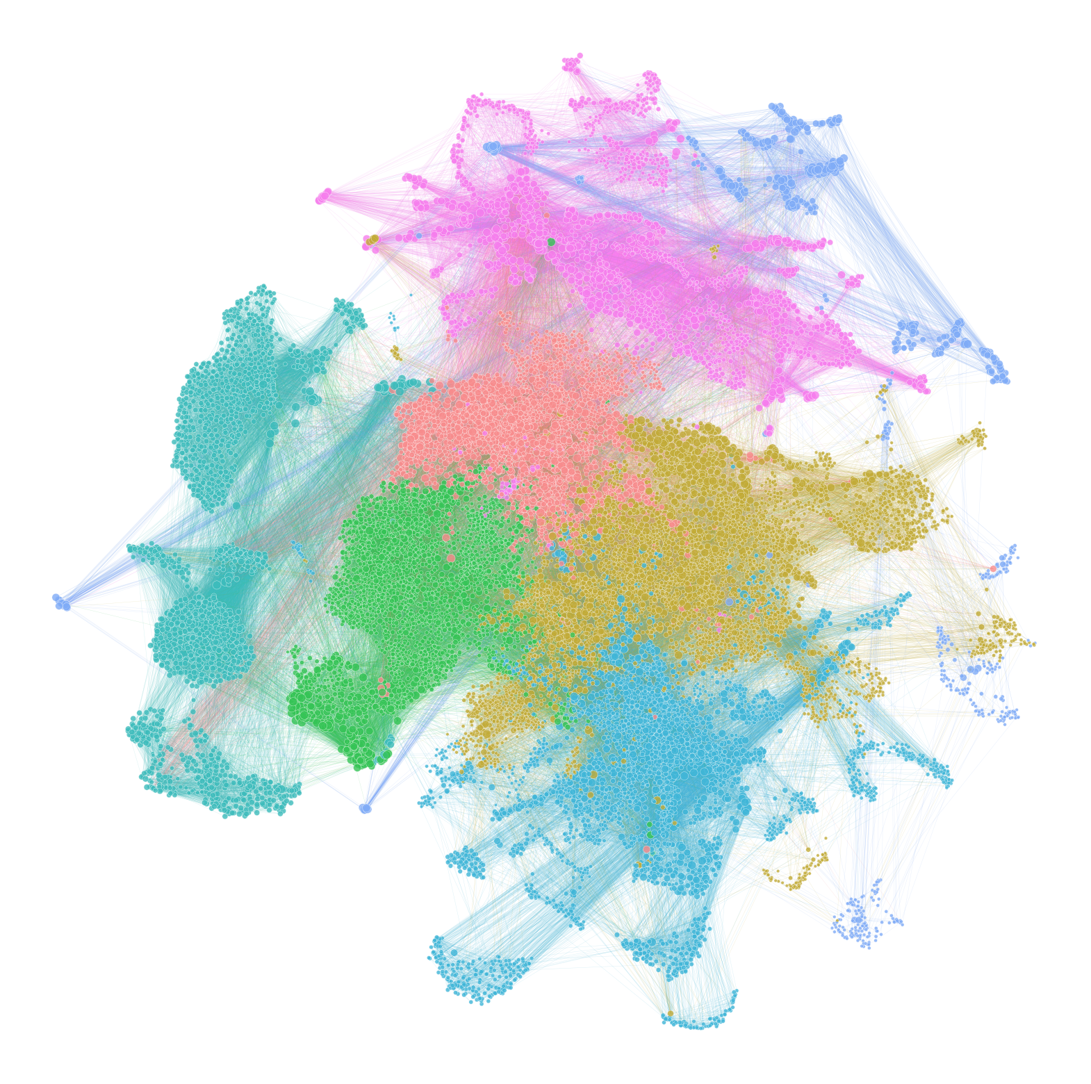
Plotting the network#
I use networkplot to generate the actual network diagram.
For very large networks, it can make things faster to subsample the number of edges which are plotted.
def subsample_edges(adjacency, n_edges_kept=100_000):
    row_inds, col_inds = np.nonzero(adjacency)
    n_edges = len(row_inds)
    if n_edges_kept > n_edges:
        return adjacency

    choice_edge_inds = np.random.choice(n_edges, size=n_edges_kept, replace=False)
    row_inds = row_inds[choice_edge_inds]
    col_inds = col_inds[choice_edge_inds]
    data = adjacency[row_inds, col_inds]

    return csr_array((data, (row_inds, col_inds)), shape=adjacency.shape)
Again, you may need to play with parameters such as node and edge sizes to get a reasonable looking plot.
from graspologic.plot import networkplot

currtime = time.time()

# this is optional, may not need depending on the number of edges you have
sub_adj = subsample_edges(adj, 100_000)

ax = networkplot(
    sub_adj,
    x="x",
    y="y",
    node_data=node_df,
    node_size="rank_strength",
    node_sizes=(10, 80),
    figsize=(20, 20),
    node_hue="community",
    edge_linewidth=0.3,
    palette=palette,
)
ax.axis("off")

print(f"{time.time() - currtime:.3f} seconds elapsed.")
1.329 seconds elapsed.