Centrality measures#
Much of this content is based heavily on Section 7.1 from Mark Newman’s “Networks” [1].
Lots of research has gone into studying various notions of a “how important is each node?” in a network. Of course, as this vague question suggests, there are many ways to define what we mean by important. Below, we’ll cover a few of the most famous and commonly used notions, primarily because it will be useful to know what these terms mean when reading studies which use network science. Also, many of these methods are based on elegant and relatively simple mathematics.
import networkx as nx
import numpy as np
from graspologic.datasets import load_drosophila_left
from graspologic.utils import binarize


A = load_drosophila_left()[:28, :28]
A = binarize(A).astype(int)
g = nx.from_numpy_array(A, create_using=nx.DiGraph)

# g = nx.karate_club_graph()

# nodelist = list(g.nodes)
# A = nx.to_numpy_array(g, nodelist=nodelist).astype(int)


def map_to_nodes(node_map):
    node_map.setdefault(0)
    # utility function to make it easy to compare dicts to array outputs
    return np.array(np.vectorize(lambda x: node_map.setdefault(x, 0))(nodelist))
Degrees#
The first notion of centrality we’ll consider is the node’s degree, sometimes called degree centrality, though I personally won’t use that term. The degree of a node is simply the number of other nodes to which it is connected.
g.degree()
DiDegreeView({0: 49, 1: 50, 2: 51, 3: 52, 4: 52, 5: 52, 6: 47, 7: 49, 8: 49, 9: 47, 10: 46, 11: 48, 12: 50, 13: 46, 14: 52, 15: 51, 16: 50, 17: 46, 18: 49, 19: 52, 20: 50, 21: 50, 22: 42, 23: 47, 24: 34, 25: 41, 26: 38, 27: 48})
degrees = dict(g.degree())
map_to_nodes(degrees)
array([49, 50, 51, 52, 52, 52, 47, 49, 49, 47, 46, 48, 50, 46, 52, 51, 50,
       46, 49, 52, 50, 50, 42, 47, 34, 41, 38, 48,  0,  0,  0,  0,  0,  0])
Computing the degree is also quite easy with the adjacency matrix (assuming the network is unweighted).
A.sum(axis=0) + A.sum(axis=1)
array([49, 50, 51, 52, 52, 52, 47, 49, 49, 47, 46, 48, 50, 46, 52, 51, 50,
       46, 49, 52, 50, 50, 42, 47, 34, 41, 38, 48])
We see that the output matches, as expected. For a directed network, there are distinct notions of degree based on whether we are considering a node’s outputs or inputs. These are simply termed out and in degree, where out degree is the number of outputs from a given node, and likewise for the in degree.
Question
If we want to compute the out degree from the adjacency matrix, should we sum along rows or along columns?
Let’s see what this looks like to compute using networkx and an adjacency matrix:
out_degrees = A.sum(axis=1)
out_degrees
array([24, 26, 26, 26, 25, 25, 24, 26, 26, 23, 25, 25, 24, 23, 25, 26, 23,
       23, 24, 25, 26, 25, 22, 24, 17, 22, 18, 21])
map_to_nodes(dict(g.out_degree()))
array([24, 26, 26, 26, 25, 25, 24, 26, 26, 23, 25, 25, 24, 23, 25, 26, 23,
       23, 24, 25, 26, 25, 22, 24, 17, 22, 18, 21,  0,  0,  0,  0,  0,  0])
in_degrees = A.sum(axis=0)
in_degrees
array([25, 24, 25, 26, 27, 27, 23, 23, 23, 24, 21, 23, 26, 23, 27, 25, 27,
       23, 25, 27, 24, 25, 20, 23, 17, 19, 20, 27])
map_to_nodes(dict(g.in_degree()))
array([25, 24, 25, 26, 27, 27, 23, 23, 23, 24, 21, 23, 26, 23, 27, 25, 27,
       23, 25, 27, 24, 25, 20, 23, 17, 19, 20, 27,  0,  0,  0,  0,  0,  0])
Eigenvector centrality#
Our next notion of importance for each node is called eigenvector centrality. The eigenvector centrality has an interesting, circular definition: nodes are considered more important if they themselves are connected to important nodes. For this and many other centrality measures, we also don’t care about the scale of these importance scores - for instance, scores of \([2, 1]\) would be interpreted the same as \([20, 10]\): the first node is twice as important as the second. We also want each of these centrality scores to be positive.
How can we write this down mathematically? Let’s say that we are after a vector \(x\), which has length \(n\) (the number of nodes in our graph). Element \(x_i\) in this vector will represent the eigenvector centrality that we are after for node \(i\). Based on what we said about in the definition, then this means that we can write:
How does this work? For any potential edge incident to \(i\) that doesn’t exist, \(A_{ij} = 0\), and thus we won’t sum up the contribution of those nodes which aren’t neighbors of \(i\). Why do we have a constant, \(c\)? Since the definition of eigenvector centrality is completely relative, we could put any constant \(c > 0\), and the definition would hold. Since this choice is relative, let’s set \(c = \frac{1}{\lambda}\), where \(\lambda\) is the largest eigenvalue of \(A\).
Now, this formula is starting to look like something we know from linear algebra. We can rewrite this set of equations (for all \(i\)) as a matrix/vector equation:
Which is the familiar definition of an eigenvector/eigenvalue, where in this case, \(x\) would correspond to the eigenvector of the largest eigenvalue of \(A\). Why are we considering only the largest eigenvalue of \(A\), rather than any other? This is because if we want a positive score for each node in our network, the only eigenvector with all positive elements will be the one we chose above, by a famous result called the Perron-Frobenius theorem.
Knowing this, we can compute the eigenvector centrality quite easily from the adjacency matrix.
g = nx.karate_club_graph()
nodelist = list(g.nodes)
A = nx.to_numpy_array(g, nodelist=nodelist)

eigenvalues, eigenvectors = np.linalg.eig(A)
first_eigenvector = np.abs(eigenvectors[:, 0])
first_eigenvector
array([0.35549144, 0.26595992, 0.3171925 , 0.21117972, 0.07596882,
       0.07948305, 0.07948305, 0.17095975, 0.22740391, 0.10267425,
       0.07596882, 0.0528557 , 0.08425463, 0.22647272, 0.10140326,
       0.10140326, 0.02363563, 0.09239954, 0.10140326, 0.14791251,
       0.10140326, 0.09239954, 0.10140326, 0.15011857, 0.05705244,
       0.05920647, 0.07557941, 0.13347715, 0.13107782, 0.13496082,
       0.1747583 , 0.19103384, 0.30864422, 0.37336347])
The eigenvector centrality is also provided as a function directly in networkx.
map_to_nodes(dict(nx.eigenvector_centrality(g)))
array([0.35548349, 0.26595387, 0.31718939, 0.21117408, 0.07596646,
       0.07948058, 0.07948058, 0.17095511, 0.22740509, 0.10267519,
       0.07596646, 0.05285417, 0.08425192, 0.2264697 , 0.10140628,
       0.10140628, 0.02363479, 0.09239676, 0.10140628, 0.14791134,
       0.10140628, 0.09239676, 0.10140628, 0.15012329, 0.05705374,
       0.0592082 , 0.07558192, 0.13347933, 0.13107926, 0.13496529,
       0.17476028, 0.19103627, 0.30865105, 0.37337121])
PageRank#
See the Wikipedia article on PageRank for more detail than I give here.
PageRank is another famous centrality measure - famous because it was one of the algorithms used early on by Google to decide which websites in a web network were important.
There are several ways to derive the definition of PageRank, but we’ll use one based on something called random walks to motivate this algorithm.
Random walks#
Note
Random walks are a very important concept in network science which we’ll come back to later in the course.
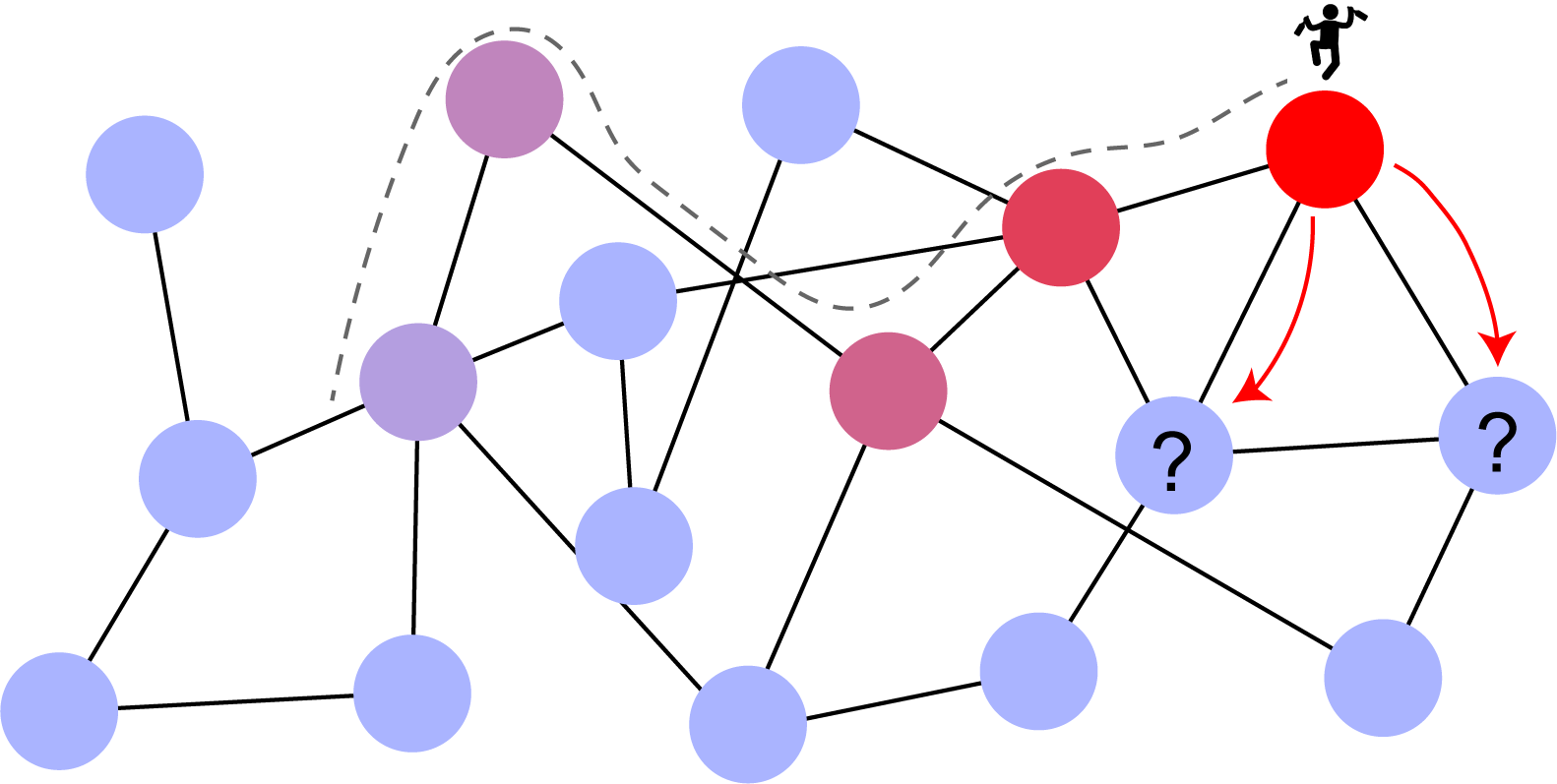
Fig. 2 Imagining a random walk on a network - image from Cesar H Comin’s website.#
Let’s say we have an unweighted, directed network (for the time being). At time \(t\), imagine you are a placed at a random node in a network, node \(i\). To decide your position at time \(t+1\), you randomly chose one of the outbound links from node \(A\) to follow.
Let \(x^{t+1}\) be an \(n\)-length vector, with all 0s except for a \(1\) at the position of our random walker at time \(t+1\).
Let \(d_{i}\) be the (out) degree of node \(i\).
We can write the probability of being at node \(j\) at time \(t+1\) as:
\(P[x_j^{t+1} = 1] = A_{ij}/d_{i}\)
In other words, this probability is \(1 / d_{i}\) if \(i\) is connected to \(j\), and 0 otherwise.
Rather than considering a single random walker (e.g. the vector \(x\) has 0’s and 1’s), it is often more useful to consider the probability distribution of a random walker. In other words, we can consider the vector \(x^{t}\) to be positive and sum to 1, and element \(x_i^{t}\) represents the probability of being at node \(i\) and time \(t\).
Let \(D\) be an \(n \times n\) matrix whose diagonal is the out degree of each node. Now, we can create a matrix \(P\) which represents the transition probabilities for our random walk:
In essence, we have just divided each row of \(A\) by its out degree.
Now, we can use a simple matrix/vector equation to update the probability distribution of our random walker at time \(t+1\) based on that at time \(t\).
Random walks with teleportation#
One issue with the model above is that sometimes a random walker could get stuck in a node with no output edges. The authors of PageRank made one small modification to this random walk scheme - at each time step, with probability \(\alpha\) the random walk proceeds as before. With probability \(1 - \alpha\), the random walker teleports to node completely at random.
Now, we have
Question
Let \(E\) be a matrix of all ones.
What is \(E x^{(t)}\)?
Hint: \(x^{(t)}\) represents a probability distribution.
We can rearrange as
Where
Given this, we are basically done finding the PageRank of each node! The logic of PageRank is simply to give an importance to each node which is proportional to the limiting probability of this random walker (with teleportation) landing on that node after a long time walking on our network. Because of some linear algebraic properties which we probably won’t get into in this course, this limiting distribution (e.g. \(x^{(t)}\) as \(t\) goes to infinity) converges in a modest number of iterations because of the teleportation probability we added. The value of \(\alpha\) can be set by the user, but typically people leave it at \(0.85\).
Below is a simple implementation of computing PageRank.
n = A.shape[0]
alpha = 0.85
n_iters = 100
out_degrees = A.sum(axis=1)
D_inv = np.diag(1 / out_degrees)
rng = np.random.default_rng()
x = rng.random(n)
x /= np.linalg.norm(x, ord=1)
P = A.T @ D_inv
P_mod = alpha * P + (1 - alpha) / n

for i in range(n_iters):
    x = P_mod @ x

x
array([0.09699729, 0.05287692, 0.05707851, 0.03585986, 0.02197795,
       0.02911115, 0.02911115, 0.0244905 , 0.02976606, 0.0143094 ,
       0.02197795, 0.00956475, 0.01464489, 0.02953646, 0.01453599,
       0.01453599, 0.01678401, 0.01455868, 0.01453599, 0.01960464,
       0.01453599, 0.01455868, 0.01453599, 0.03152251, 0.02107603,
       0.0210062 , 0.01504404, 0.02563977, 0.01957346, 0.02628854,
       0.02459016, 0.03715809, 0.07169323, 0.10091918])
Tip
A good exercise would be to plot how much this vector (x) is changing between each iteration.
How long does it take for this process to converge? Or, what happens if you use a different
initialization?
Note that this is algorithm also has an interpretation as finding the principal eigenvector
of the matrix P_mod above through a process known as power iteration.
eigenvalues, eigenvectors = np.linalg.eig(P_mod)
first_eigenvector = np.abs(eigenvectors[:, 0])
first_eigenvector /= np.linalg.norm(first_eigenvector, ord=1)
first_eigenvector
array([0.09699729, 0.05287692, 0.05707851, 0.03585986, 0.02197795,
       0.02911115, 0.02911115, 0.0244905 , 0.02976606, 0.0143094 ,
       0.02197795, 0.00956475, 0.01464489, 0.02953646, 0.01453599,
       0.01453599, 0.01678401, 0.01455868, 0.01453599, 0.01960464,
       0.01453599, 0.01455868, 0.01453599, 0.03152251, 0.02107603,
       0.0210062 , 0.01504404, 0.02563977, 0.01957346, 0.02628854,
       0.02459016, 0.03715809, 0.07169323, 0.10091918])
The algorithms we used above get very similar answers to the version implemented in networkx. There are a couple of parameters (max iterations, stopping tolerance, initial distribution) which can affect the results slightly.
pagerank_dict = nx.pagerank(g, max_iter=100)
np.vectorize(pagerank_dict.get)(nodelist)
array([0.09700182, 0.05287839, 0.05707842, 0.03586064, 0.02197941,
       0.02911334, 0.02911334, 0.02449076, 0.02976534, 0.01430895,
       0.02197941, 0.00956492, 0.01464519, 0.02953631, 0.01453516,
       0.01453516, 0.01678538, 0.01455886, 0.01453516, 0.01960442,
       0.01453516, 0.01455886, 0.01453516, 0.03152092, 0.02107546,
       0.02100563, 0.0150434 , 0.0256388 , 0.01957296, 0.02628726,
       0.02458934, 0.03715664, 0.07169213, 0.10091792])
Betweenness centrality#
Shortest paths#
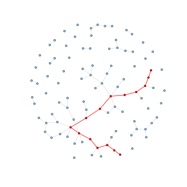
Fig. 3 Illustration of a shortest path between two nodes. Image from Shortest paths.#
Rather than considering random walks, betweenness centrality is based on shortest paths. A shortest path between node \(i\) and node \(j\) is a path (a sequence of edges to traverse) which uses as few edges as possible to get from \(i\) to \(j\). If you’d like to compute shortest paths with a sparse adjacency matrix, you can do this in scipy using scipy.sparse.csgraph.shortest_path. In networkx, you can use shortest_path and several other similar functions.
Motivating betweenness centrality#
Betweenness centrality uses the following motivation: imaging we have a network where every pair of nodes needs to exchange information. Further, we assume that each node is equally efficient at transmitting information, and that information will flow between pairs of nodes using the shortest path.
Betweenness centrality, then, is based on the following simple logic: a node is more important if more information passes through them. In other words, the betweenness centrality of node \(i\) is proportional to the number of these shortest paths (among all other nodes) which contain \(i\).
Let’s say that \(n^{i}_{st}\) is an indicator, where it is 1 if node \(i\) is on the shortest path from \(s\) to \(t\) and 0 otherwise.
We can then write the betweenness centrality of node \(i\), \(x_i\), as
There are a few modifications which are usually made to the formula above - for instance, if there are multiple shortest paths between \(s\) and \(t\), we would divide \(n_{st}^i\) by how many paths there are, \(g_{st}\). And, some will normalize the path count by the number of possible paths to make betweenness the fraction of paths running through that node. So, we end up with
n = len(g)
betweenness = np.zeros(n)

all_paths = nx.shortest_path(g)
for source_node, path_collection in all_paths.items():
    for target_node, path in path_collection.items():
        for node in path[1:-1]:  # ignore the start and end nodes themselves
            betweenness[node] += 1 / n**2

betweenness
array([0.45934256, 0.02595156, 0.26816609, 0.        , 0.        ,
       0.05190311, 0.0017301 , 0.        , 0.03979239, 0.        ,
       0.        , 0.        , 0.        , 0.00692042, 0.        ,
       0.        , 0.        , 0.        , 0.        , 0.        ,
       0.        , 0.        , 0.        , 0.02768166, 0.0017301 ,
       0.01384083, 0.        , 0.03373702, 0.        , 0.00692042,
       0.        , 0.06747405, 0.23442907, 0.12716263])
map_to_nodes(nx.betweenness_centrality(g))
array([0.43763528, 0.05393669, 0.14365681, 0.01190927, 0.00063131,
       0.02998737, 0.02998737, 0.        , 0.05592683, 0.00084776,
       0.00063131, 0.        , 0.        , 0.0458634 , 0.        ,
       0.        , 0.        , 0.        , 0.        , 0.03247505,
       0.        , 0.        , 0.        , 0.01761364, 0.0022096 ,
       0.00384049, 0.        , 0.02233345, 0.00179473, 0.00292208,
       0.01441198, 0.13827561, 0.14524711, 0.30407498])
Note
My simple implementation does not properly deal with the case where there is
more than one shortest path between two nodes, and networkx also uses a slightly different
normalization constant than I did. I believe these two factors cause the slight difference
in results.
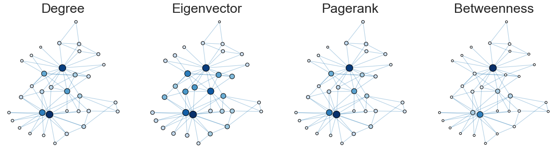
Comparing the centrality measures#
Let’s compare how these different notions of centrality look on this network.
import pandas as pd
import matplotlib.pyplot as plt
from graspologic.plot import networkplot
import seaborn as sns
from matplotlib import colors

node_data = pd.DataFrame(index=g.nodes())
node_data["degree"] = node_data.index.map(dict(nx.degree(g)))
node_data["eigenvector"] = node_data.index.map(nx.eigenvector_centrality(g))
node_data["pagerank"] = node_data.index.map(nx.pagerank(g))
node_data["betweenness"] = node_data.index.map(nx.betweenness_centrality(g))

pos = nx.kamada_kawai_layout(g)
node_data["x"] = [pos[node][0] for node in node_data.index]
node_data["y"] = [pos[node][1] for node in node_data.index]

sns.set_context("talk", font_scale=1.5)
fig, axs = plt.subplots(1, 4, figsize=(20, 5))


def plot_node_scaled_network(A, node_data, key, ax):
    # REF: https://github.com/mwaskom/seaborn/blob/9425588d3498755abd93960df4ab05ec1a8de3ef/seaborn/_core.py#L215

    levels = list(np.sort(node_data[key].unique()))
    cmap = sns.color_palette("Blues", as_cmap=True)
    vmin = np.min(levels)
    norm = colors.Normalize(vmin=0.3 * vmin)
    palette = dict(zip(levels, cmap(norm(levels))))

    networkplot(
        A,
        node_data=node_data,
        x="x",
        y="y",
        ax=ax,
        edge_linewidth=1.0,
        node_size=key,
        node_hue=key,
        palette=palette,
        node_sizes=(20, 200),
        node_kws=dict(linewidth=1, edgecolor="black"),
        node_alpha=1.0,
        edge_kws=dict(color=sns.color_palette()[0]),
    )

    ax.axis("off")
    ax.set_title(key.capitalize())


ax = axs[0]
plot_node_scaled_network(A, node_data, "degree", ax)

ax = axs[1]
plot_node_scaled_network(A, node_data, "eigenvector", ax)

ax = axs[2]
plot_node_scaled_network(A, node_data, "pagerank", ax)

ax = axs[3]
plot_node_scaled_network(A, node_data, "betweenness", ax)

fig.set_facecolor("w")
node_data
| degree | eigenvector | pagerank | betweenness | x | y | |
|---|---|---|---|---|---|---|
| 0 | 16 | 0.355483 | 0.097002 | 0.437635 | 0.025953 | 0.332618 |
| 1 | 9 | 0.265954 | 0.052878 | 0.053937 | -0.154154 | 0.251060 |
| 2 | 10 | 0.317189 | 0.057078 | 0.143657 | 0.072811 | -0.003398 |
| 3 | 6 | 0.211174 | 0.035861 | 0.011909 | 0.151208 | 0.232506 |
| 4 | 3 | 0.075966 | 0.021979 | 0.000631 | 0.193135 | 0.574454 |
| 5 | 4 | 0.079481 | 0.029113 | 0.029987 | 0.189964 | 0.679017 |
| 6 | 4 | 0.079481 | 0.029113 | 0.029987 | -0.004422 | 0.691958 |
| 7 | 4 | 0.170955 | 0.024491 | 0.000000 | 0.283520 | 0.210236 |
| 8 | 5 | 0.227405 | 0.029765 | 0.055927 | -0.175658 | -0.009901 |
| 9 | 2 | 0.102675 | 0.014309 | 0.000848 | 0.070613 | -0.289252 |
| 10 | 3 | 0.075966 | 0.021979 | 0.000631 | 0.379808 | 0.532623 |
| 11 | 1 | 0.052854 | 0.009565 | 0.000000 | -0.187765 | 0.633252 |
| 12 | 2 | 0.084252 | 0.014645 | 0.000000 | 0.433744 | 0.379505 |
| 13 | 5 | 0.226470 | 0.029536 | 0.045863 | -0.085120 | 0.052682 |
| 14 | 2 | 0.101406 | 0.014535 | 0.000000 | -0.500067 | -0.312444 |
| 15 | 2 | 0.101406 | 0.014535 | 0.000000 | -0.465779 | -0.429025 |
| 16 | 2 | 0.023635 | 0.016785 | 0.000000 | 0.159578 | 1.000000 |
| 17 | 2 | 0.092397 | 0.014559 | 0.000000 | -0.279331 | 0.514205 |
| 18 | 2 | 0.101406 | 0.014535 | 0.000000 | -0.395900 | -0.534397 |
| 19 | 3 | 0.147911 | 0.019604 | 0.032475 | -0.275385 | 0.069220 |
| 20 | 2 | 0.101406 | 0.014535 | 0.000000 | -0.293375 | -0.615543 |
| 21 | 2 | 0.092397 | 0.014559 | 0.000000 | -0.373191 | 0.436351 |
| 22 | 2 | 0.101406 | 0.014535 | 0.000000 | -0.158642 | -0.642802 |
| 23 | 5 | 0.150123 | 0.031521 | 0.017614 | 0.236065 | -0.515501 |
| 24 | 3 | 0.057054 | 0.021075 | 0.002210 | 0.570081 | -0.296654 |
| 25 | 3 | 0.059208 | 0.021006 | 0.003840 | 0.548790 | -0.166394 |
| 26 | 2 | 0.075582 | 0.015043 | 0.000000 | -0.047563 | -0.757920 |
| 27 | 4 | 0.133479 | 0.025639 | 0.022333 | 0.284627 | -0.289822 |
| 28 | 3 | 0.131079 | 0.019573 | 0.001795 | 0.185397 | -0.292763 |
| 29 | 4 | 0.134965 | 0.026287 | 0.002922 | 0.068520 | -0.620426 |
| 30 | 4 | 0.174760 | 0.024589 | 0.014412 | -0.381375 | -0.089401 |
| 31 | 6 | 0.191036 | 0.037157 | 0.138276 | 0.197179 | -0.072189 |
| 32 | 12 | 0.308651 | 0.071692 | 0.145247 | -0.172313 | -0.312215 |
| 33 | 17 | 0.373371 | 0.100918 | 0.304075 | -0.100954 | -0.339640 |
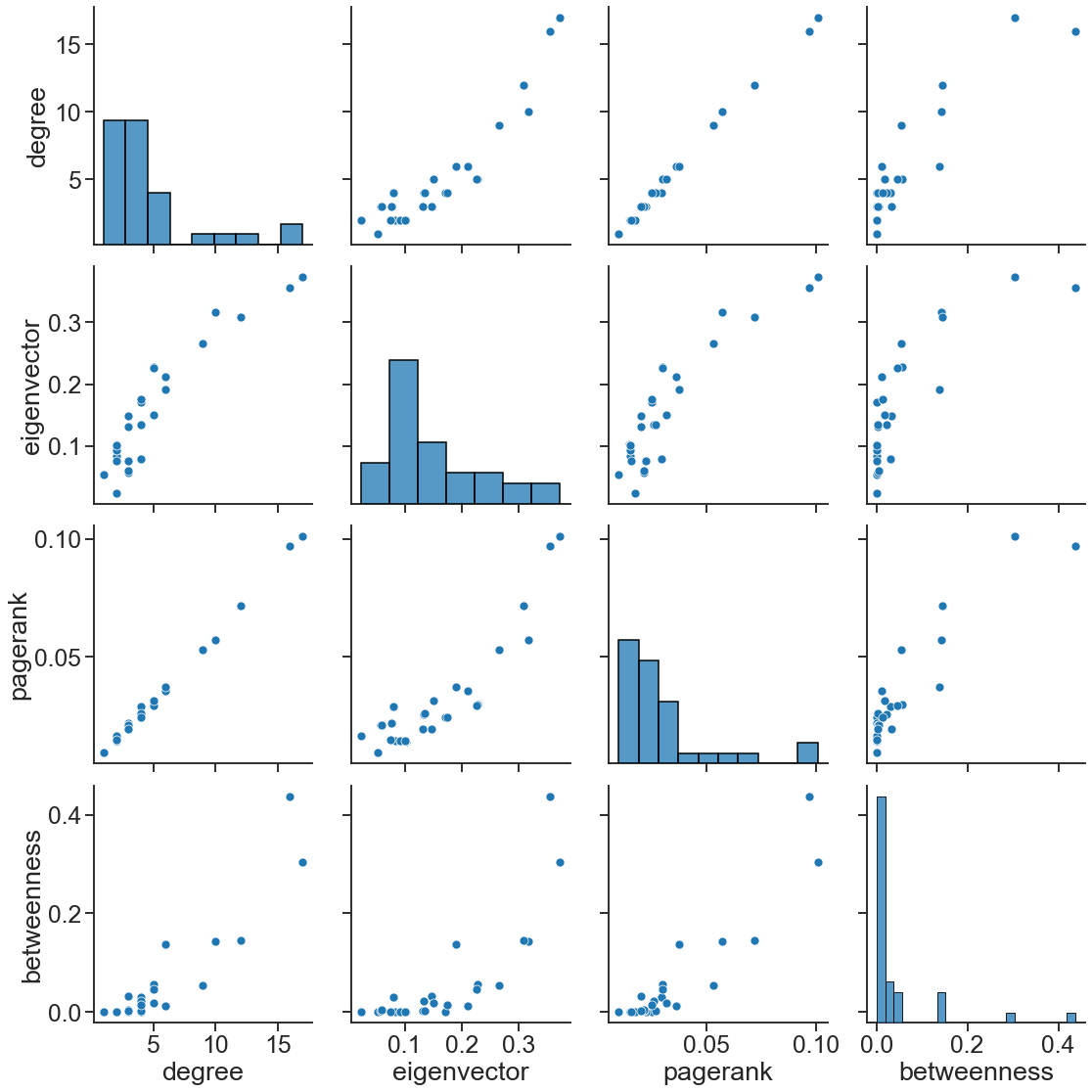
We can look at how correlated each of these measures are, but keep in mind, this may look very different on different networks!
sns.pairplot(
    node_data, vars=["degree", "eigenvector", "pagerank", "betweenness"], height=4
)
<seaborn.axisgrid.PairGrid at 0x143259b50>
Final note#
Please keep in mind that there are many, many more notions of centrality that we didn’t
go into here. More of these are described in Section 7.1 from Mark Newman’s “Networks”
[1], as well as the centrality section in networkx’s documentation.